


![[The AI Show Episode 146]: Rise of “AI-First” Companies, AI Job Disruption, GPT-4o Update Gets Rolled Back, How Big Consulting Firms Use AI, and Meta AI App](https://www.marketingaiinstitute.com/hubfs/ep%20146%20cover.png)


![Beats Studio Pro Wireless Headphones Now Just $169.95 - Save 51%! [Deal]](https://www.iclarified.com/images/news/97258/97258/97258-640.jpg)


HTAP Using a Star Query on MongoDB Atlas Search Index
MongoDB is used for its strength in managing online transaction processing (OLTP) with a document model that naturally aligns with domain-specific transactions and their access patterns. In addition to these capabilities, MongoDB supports advanced search techniques through its Atlas Search index, based on Apache Lucene. This can be used for near-real-time analytics and, combined with aggregation pipeline, add some online analytical processing (OLAP) capabilities. Thanks to the document model, this analytics capability doesn't require a different data structure and enables MongoDB to execute hybrid transactional and analytical (HTAP) workloads efficiently, as demonstrated in this article with an example from a healthcare domain. Traditional relational databases employ a complex query optimization method known as "star transformation" and rely on multiple single-column indexes, along with bitmap operations, for efficient ad-hoc queries. This requires a dimensional schema, or star schema, which differs from the normalized operational schema updated by transactions. In contrast, MongoDB can be queried with a similar strategy using its document schema for operational use cases, simply requiring the addition of an Atlas Search index on the collection that stores transaction facts. To demonstrate how a single index on a fact collection enables efficient queries even when filters are applied to other dimension collections, I utilize the MedSynora DW dataset, which is similar to a star schema with dimensions and facts. This dataset, published by M. Ebrar Küçük on Kaggle, is a synthetic hospital data warehouse covering patient encounters, treatments, and lab tests, and is compliant with privacy standards for healthcare data science and machine learning. Import the dataset The dataset is accessible on Kaggle as a folder of comma-separated values (CSV) files for dimensions and facts compressed into a 730MB zip file. The largest fact table that I'll use holds 10 million records. I download the CSV files and uncompress them: curl -L -o medsynora-dw.zip "https://www.kaggle.com/api/v1/datasets/download/mebrar21/medsynora-dw" unzip medsynora-dw.zip I import each file into a collection, using mongoimport from the MongoDB Database Tools: for i in "MedSynora DW"/*.csv do mongoimport -d "MedSynoraDW" --file="$i" --type=csv --headerline -c "$(basename "$i" .csv)" -j 8 done For this demo, I'm interested in two fact tables: FactEncounter and FactLabTest. Here are the fields described in the file headers: # head -1 "MedSynora DW"/Fact{Encounter,LabTests}.csv ==> MedSynora DW/FactEncounter.csv MedSynora DW/FactLabTests.csv MedSynora DW/DimDisease.csv MedSynora DW/DimDoctor.csv MedSynora DW/DimInsurance.csv MedSynora DW/DimPatient.csv MedSynora DW/DimRoom.csv doc["Patient_ID"]).toArray() } // Primary Key in Dimension }) The following adds the conditions on the Doctor (Japanese): search["$search"]["compound"]["must"].push( { in: { path: "ResponsibleDoctorID", // Foreign Key in Fact value: db.DimDoctor.find( // Dimension collection {"Doctor Nationality": "Japanese" } // filter on Dimension ).map(doc => doc["Doctor_ID"]).toArray() } // Primary Key in Dimension }) The following adds the condition on the Room (Deluxe): search["$search"]["compound"]["must"].push( { in: { path: "RoomKey", // Foreign Key in Fact value: db.DimRoom.find( // Dimension collection {"Room Type": "Deluxe" } // filter on Dimension ).map(doc => doc["RoomKey"]).toArray() } // Primary Key in Dimension }) The following adds the condition on the Disease (Hematology): search["$search"]["compound"]["must"].push( { in: { path: "Disease_ID", // Foreign Key in Fact value: db.DimDisease.find( // Dimension collection {"Disease Type": "Hematology" } // filter on Dimension ).map(doc => doc["Disease_ID"]).toArray() } // Primary Key in Dimension }) Finally, the condition on the Insurance coverage (greater than 80%): search["$search"]["compound"]["must"].push( { in: { path: "InsuranceKey", // Foreign Key in Fact value: db.DimInsurance.find( // Dimension collection {"Coverage Limit": { "$gt": 0.8 } } // filter on Dimension ).map(doc => doc["InsuranceKey"]).toArray() } // Primary Key in Dimension }) All these search criteria have the same shape: a find() on the dimension collection, with the filters from the query, resulting in an array of dimension keys (like a primary key in a dimension table) that are used to search in the fact documents using it as a reference (like a foreign key in a fact table). Each of those steps has queried the dimension collection to obtain a simple array of dimension keys, which are added to the aggrega

MongoDB is used for its strength in managing online transaction processing (OLTP) with a document model that naturally aligns with domain-specific transactions and their access patterns. In addition to these capabilities, MongoDB supports advanced search techniques through its Atlas Search index, based on Apache Lucene. This can be used for near-real-time analytics and, combined with aggregation pipeline, add some online analytical processing (OLAP) capabilities. Thanks to the document model, this analytics capability doesn't require a different data structure and enables MongoDB to execute hybrid transactional and analytical (HTAP) workloads efficiently, as demonstrated in this article with an example from a healthcare domain.
Traditional relational databases employ a complex query optimization method known as "star transformation" and rely on multiple single-column indexes, along with bitmap operations, for efficient ad-hoc queries. This requires a dimensional schema, or star schema, which differs from the normalized operational schema updated by transactions. In contrast, MongoDB can be queried with a similar strategy using its document schema for operational use cases, simply requiring the addition of an Atlas Search index on the collection that stores transaction facts.
To demonstrate how a single index on a fact collection enables efficient queries even when filters are applied to other dimension collections, I utilize the MedSynora DW dataset, which is similar to a star schema with dimensions and facts. This dataset, published by M. Ebrar Küçük on Kaggle, is a synthetic hospital data warehouse covering patient encounters, treatments, and lab tests, and is compliant with privacy standards for healthcare data science and machine learning.
Import the dataset
The dataset is accessible on Kaggle as a folder of comma-separated values (CSV) files for dimensions and facts compressed into a 730MB zip file. The largest fact table that I'll use holds 10 million records.
I download the CSV files and uncompress them:
curl -L -o medsynora-dw.zip "https://www.kaggle.com/api/v1/datasets/download/mebrar21/medsynora-dw"

unzip medsynora-dw.zip
I import each file into a collection, using mongoimport from the MongoDB Database Tools:
for i in "MedSynora DW"/*.csv
do
 mongoimport -d "MedSynoraDW" --file="$i"  --type=csv --headerline -c "$(basename "$i" .csv)" -j 8
done
For this demo, I'm interested in two fact tables: FactEncounter and FactLabTest. Here are the fields described in the file headers:
# head -1 "MedSynora DW"/Fact{Encounter,LabTests}.csv

==> MedSynora DW/FactEncounter.csv <==
Encounter_ID,Patient_ID,Disease_ID,ResponsibleDoctorID,InsuranceKey,RoomKey,CheckinDate,CheckoutDate,CheckinDateKey,CheckoutDateKey,Patient_Severity_Score,RadiologyType,RadiologyProcedureCount,EndoscopyType,EndoscopyProcedureCount,CompanionPresent

==> MedSynora DW/FactLabTests.csv <==
Encounter_ID,Patient_ID,Phase,LabType,TestName,TestValue
The fact tables reference the following dimensions:
# head -1 "MedSynora DW"/Dim{Disease,Doctor,Insurance,Patient,Room}.csv

==> MedSynora DW/DimDisease.csv <==
Disease_ID,Admission Diagnosis,Disease Type,Disease Severity,Medical Unit

==> MedSynora DW/DimDoctor.csv <==
Doctor_ID,Doctor Name,Doctor Surname,Doctor Title,Doctor Nationality,Medical Unit,Max Patient Count

==> MedSynora DW/DimInsurance.csv <==
InsuranceKey,Insurance Plan Name,Coverage Limit,Deductible,Excluded Treatments,Partial Coverage Treatments

==> MedSynora DW/DimPatient.csv <==
Patient_ID,First Name,Last Name,Gender,Birth Date,Height,Weight,Marital Status,Nationality,Blood Type

==> MedSynora DW/DimRoom.csv <==
RoomKey,Care_Level,Room Type
Here is the dimensional model, often referred to as a "star schema" because the fact tables are located at the center, referencing the dimensions. Because of normalization, when facts contain a one-to-many composition it is described in two CSV files to fit into two SQL tables:
Star schema with facts and dimensions. The facts are stored in two tables in CSV files or a SQL database, but on a single collection in MongoDB. It holds the fact measures and dimension keys, which reference the key of the dimension collections.
MongoDB allows the storage of one-to-many compositions, such as Encounters and LabTests, within a single collection. By embedding LabTests as an array in Encounter documents, this design pattern promotes data colocation to reduce disk access and increase cache locality, minimizes duplication to improve storage efficiency, maintains data integrity without requiring additional foreign key processing, and enables more indexing possibilities. The document model also circumvents a common issue in SQL analytic queries, where joining prior to aggregation may yield inaccurate results due to the repetition of parent values in a one-to-many relationship.
As this would be the right data model for an operational database with such data, I create a new collection, using an aggregation pipeline, that I'll use instead of the two that were imported from the normalized CSV:
db.FactLabTests.createIndex({ Encounter_ID: 1, Patient_ID: 1 });

db.FactEncounter.aggregate([
  {
    $lookup: {
      from: "FactLabTests",
      localField: "Encounter_ID",
      foreignField: "Encounter_ID",
      as: "LabTests"
    }
  },
  {
    $addFields: {
      LabTests: {
        $map: {
          input: "$LabTests",
          as: "test",
          in: {
            Phase: "$$test.Phase",
            LabType: "$$test.LabType",
            TestName: "$$test.TestName",
            TestValue: "$$test.TestValue"
          }
        }
      }
    }
  },
  {
    $out: "FactEncounterLabTests"
  }
]);
Here is how one document looks:
AtlasLocalDev atlas [direct: primary] MedSynoraDW>

db.FactEncounterLabTests.find().limit(1)
[
  {
    _id: ObjectId('67fc3d2f40d2b3c843949c97'),
    Encounter_ID: 2158,
    Patient_ID: 'TR479',
    Disease_ID: 1632,
    ResponsibleDoctorID: 905,
    InsuranceKey: 82,
    RoomKey: 203,
    CheckinDate: '2024-01-23 11:09:00',
    CheckoutDate: '2024-03-29 17:00:00',
    CheckinDateKey: 20240123,
    CheckoutDateKey: 20240329,
    Patient_Severity_Score: 63.2,
    RadiologyType: 'None',
    RadiologyProcedureCount: 0,
    EndoscopyType: 'None',
    EndoscopyProcedureCount: 0,
    CompanionPresent: 'True',
    LabTests: [
      {
        Phase: 'Admission',
        LabType: 'CBC',
        TestName: 'Lymphocytes_abs (10^3/µl)',
        TestValue: 1.34
      },
      {
        Phase: 'Admission',
        LabType: 'Chem',
        TestName: 'ALT (U/l)',
        TestValue: 20.5
      },
      {
        Phase: 'Admission',
        LabType: 'Lipids',
        TestName: 'Triglycerides (mg/dl)',
        TestValue: 129.1
      },
      {
        Phase: 'Discharge',
        LabType: 'CBC',
        TestName: 'RBC (10^6/µl)',
        TestValue: 4.08
      },
...
In MongoDB, the document model utilizes embedding and reference design patterns, resembling a star schema with a primary fact collection and references to various dimension collections. It is crucial to ensure that the dimension references are properly indexed before querying these collections.
Atlas Search index
Search indexes are distinct from regular indexes, which rely on a single composite key, as they can index multiple fields without requiring a specific order to establish a key. This feature makes them perfect for ad-hoc queries, where the filtering dimensions are not predetermined.
I create a single Atlas Search index that encompasses all dimensions or measures that I might use in predicates, including those found in an embedded document:
db.FactEncounterLabTests.createSearchIndex(
  "SearchFactEncounterLabTests", {
    mappings: {
      dynamic: false,
      fields: {
        "Encounter_ID":        { "type": "number"  },
        "Patient_ID":          { "type": "token"  },
        "Disease_ID":          { "type": "number"  },
        "InsuranceKey":        { "type": "number"  },
        "RoomKey":             { "type": "number"  },
        "ResponsibleDoctorID": { "type": "number" },
        "CheckinDate":         { "type": "token"  },
        "CheckoutDate":        { "type": "token"  },
        "LabTests":            {
          "type": "document" , fields: {
            "Phase":           { "type": "token"  },
            "LabType":         { "type": "token"  },
            "TestName":        { "type": "token"  },
            "TestValue":       { "type": "number" }
          }
        }
      }
    }
  }
);
Since I don't need extra text searching on the keys, I designate the character string ones as token. I label the integer keys as number. Generally, the keys are utilized for equality predicates. However, some can be employed for ranges when the format permits, such as check-in and check-out dates formatted as YYYY-MM-DD.
In a relational database, the star schema approach emphasizes the importance of limiting the number of columns in the fact tables, as they typically contain numerous rows. Smaller dimension tables can hold more columns and are typically denormalized in SQL databases (favoring a star schema over a snowflake schema). Likewise, in document modeling, incorporating all dimension fields would unnecessarily increase the size of the fact collection documents, making it more straightforward to reference the dimension collection. The general principles of data modeling in MongoDB enable querying it as a star schema without requiring extra consideration, as MongoDB databases are designed for the application access patterns.
Star query
A star schema allows processing queries which filter fields within dimension collections in several stages:
- In the first stage, filters are applied to the dimension collections to extract all dimension keys. These keys typically do not require additional indexes, as the dimensions are generally small in size.
- In the second stage, a search is conducted using all previously obtained dimension keys on the fact collection. This process utilizes the search index built on those keys, allowing for quick access to the required documents.
- A third stage may retrieve additional dimensions to gather the necessary fields for aggregation or projection. This multi-stage process ensures that the applied filter reduces the dataset from the large fact collection before any further operations are conducted.
For an example query, I aim to analyze lab test records for female patients who are over 170 cm tall, underwent lipid lab tests, have insurance coverage exceeding 80%, and were treated by Japanese doctors in deluxe rooms for hematological conditions.
Search aggregation pipeline
To optimize the fact collection process and apply all filters, I will begin with a simple aggregation pipeline that starts with a search on the search index. This allows for filters to be applied directly to the fact collection's fields, while additional filters will be incorporated in stage one of the star query. I utilize a local variable with a compound operator to facilitate the addition of more filters for each dimension in stage one of the star query.
Before going though the star query stages to add filters on dimensions, my query has a filter on the lab type which is in the fact collection, and indexed.
const search =  {
    "$search": {
      "index": "SearchFactEncounterLabTests",
      "compound": {
        "must": [
          { "in":    { "path": "LabTests.LabType" , "value": "Lipids"   } },
        ]
      },
      "sort": { CheckoutDate: -1 }
    }
  }
I have added a "sort" operation to sort the result by check-out date in descending order. This illustrates the advantage of sorting during the index search rather than in later steps of the aggregation pipeline, particularly when a "limit" is applied.
I'll use this local variable to add more filters in Stage 1 of the star query, so that it can be executed for Stage 2, and collect documents for Stage 3.
Stage 1: Query the dimension collections
In the first phase of the star query, I obtain the dimension keys from the dimension collections. For every dimension with a filter, get the dimension keys, with a find() on the dimension, and append a "must" condition to the "compound" of the fact index search.
The following adds the conditions on the Patient (female patients over 170 cm):
search["$search"]["compound"]["must"].push( { in: {
 path: "Patient_ID",                         // Foreign Key in Fact
 value: db.DimPatient.find(                  // Dimension collection
  {Gender: "Female", Height: { "$gt": 170 }} // filter on Dimension
 ).map(doc => doc["Patient_ID"]).toArray() } // Primary Key in Dimension
})
The following adds the conditions on the Doctor (Japanese):
search["$search"]["compound"]["must"].push( { in: {
 path: "ResponsibleDoctorID",               // Foreign Key in Fact
 value: db.DimDoctor.find(                  // Dimension collection
  {"Doctor Nationality": "Japanese" }       // filter on Dimension
 ).map(doc => doc["Doctor_ID"]).toArray() } // Primary Key in Dimension
})
The following adds the condition on the Room (Deluxe):
search["$search"]["compound"]["must"].push( { in: {
 path: "RoomKey",                         // Foreign Key in Fact
 value: db.DimRoom.find(                  // Dimension collection
  {"Room Type": "Deluxe" }                // filter on Dimension
 ).map(doc => doc["RoomKey"]).toArray() } // Primary Key in Dimension
})
The following adds the condition on the Disease (Hematology):
search["$search"]["compound"]["must"].push( { in: {
 path: "Disease_ID",                         // Foreign Key in Fact
 value: db.DimDisease.find(                  // Dimension collection
  {"Disease Type": "Hematology" } // filter on Dimension
 ).map(doc => doc["Disease_ID"]).toArray() } // Primary Key in Dimension
})
Finally, the condition on the Insurance coverage (greater than 80%):
search["$search"]["compound"]["must"].push( { in: {
 path: "InsuranceKey",                         // Foreign Key in Fact
 value: db.DimInsurance.find(                  // Dimension collection
  {"Coverage Limit": { "$gt": 0.8 } }          // filter on Dimension
 ).map(doc => doc["InsuranceKey"]).toArray() } // Primary Key in Dimension
})
All these search criteria have the same shape: a find() on the dimension collection, with the filters from the query, resulting in an array of dimension keys (like a primary key in a dimension table) that are used to search in the fact documents using it as a reference (like a foreign key in a fact table).
Each of those steps has queried the dimension collection to obtain a simple array of dimension keys, which are added to the aggregation pipeline. Rather than joining tables like in a relational database, the criteria on the dimensions are pushed down to the query on the fact tables.
Stage 2: Query the fact search index
With short queries on the dimensions, I have built the following pipeline search step:
AtlasLocalDev atlas [direct: primary] MedSynoraDW> print(search)
{
  '$search': {
    index: 'SearchFactEncounterLabTests',
    compound: {
      must: [
        { in: { path: 'LabTests.LabType', value: 'Lipids' } },
        {
          in: {
            path: 'Patient_ID',
            value: [
              'TR551',    'TR751',    'TR897',    'TRGT201',  'TRJB261',
              'TRQG448',  'TRSQ510',  'TRTP535',  'TRUC548',  'TRVT591',
              'TRABU748', 'TRADD783', 'TRAZG358', 'TRBCI438', 'TRBTY896',
              'TRBUH905', 'TRBXU996', 'TRCAJ063', 'TRCIM274', 'TRCXU672',
              'TRDAB731', 'TRDFZ885', 'TRDGE890', 'TRDJK974', 'TRDKN003',
              'TRE004',   'TRMN351',  'TRRY492',  'TRTI528',  'TRAKA962',
              'TRANM052', 'TRAOY090', 'TRARY168', 'TRASU190', 'TRBAG384',
              'TRBYT021', 'TRBZO042', 'TRCAS072', 'TRCBF085', 'TRCOB419',
              'TRDMD045', 'TRDPE124', 'TRDWV323', 'TREUA926', 'TREZX079',
              'TR663',    'TR808',    'TR849',    'TRKA286',  'TRLC314',
              'TRMG344',  'TRPT435',  'TRVZ597',  'TRXC626',  'TRACT773',
              'TRAHG890', 'TRAKW984', 'TRAMX037', 'TRAQR135', 'TRARX167',
              'TRARZ169', 'TRASW192', 'TRAZN365', 'TRBDW478', 'TRBFG514',
              'TRBOU762', 'TRBSA846', 'TRBXR993', 'TRCRL507', 'TRDKA990',
              'TRDKD993', 'TRDTO238', 'TRDSO212', 'TRDXA328', 'TRDYU374',
              'TRDZS398', 'TREEB511', 'TREVT971', 'TREWZ003', 'TREXW026',
              'TRFVL639', 'TRFWE658', 'TRGIZ991', 'TRGVK314', 'TRGWY354',
              'TRHHV637', 'TRHNS790', 'TRIMV443', 'TRIQR543', 'TRISL589',
              'TRIWQ698', 'TRIWL693', 'TRJDT883', 'TRJHH975', 'TRJHT987',
              'TRJIM006', 'TRFVZ653', 'TRFYQ722', 'TRFZY756', 'TRGNZ121',
              ... 6184 more items
            ]
          }
        },
        {
          in: {
            path: 'ResponsibleDoctorID',
            value: [ 830, 844, 862, 921 ]
          }
        },
        { in: { path: 'RoomKey', value: [ 203 ] } },
        {
          in: {
            path: 'Disease_ID',
            value: [
              1519, 1506, 1504, 1510,
              1515, 1507, 1503, 1502,
              1518, 1517, 1508, 1513,
              1509, 1512, 1516, 1511,
              1505, 1514
            ]
          }
        },
        { in: { path: 'InsuranceKey', value: [ 83, 84 ] } }
      ]
    },
    sort: { CheckoutDate: -1
  }
}
MongoDB Atlas Search indexes, built on Apache Lucene, efficiently handle complex queries with multiple conditions and manage long arrays of values. In this example, a search operation integrates the compound operator with the "must" clause to apply filters across attributes. This capability simplifies query design after resolving complex filters into lists of dimension keys.
With the "search" operation created above, I can run an aggregation pipeline to get the document I'm interested in:
db.FactEncounterLabTests.aggregate([
 search,
])
With my example, nine documents are returned in 50 milliseconds.
Estimate the count
This approach is ideal for queries with filters on many conditions, where none are very selective alone, but the combination is highly selective. Using queries on dimensions and a search index on facts avoids reading more documents than necessary. However, depending on the operations you will add to the aggregation pipeline, it is a good idea to estimate the number of records returned by the search index to avoid runaway queries.
Typically, an application that allows users to execute multi-criteria queries may define a threshold and return an error or warning when the estimated number of documents exceeds it, prompting the user to add more filters. For such cases, you can run a "$searchMeta" on the index before a "$search" operation. For example, the following checks that the number of documents returned by the filter is lower than 10,000:
MedSynoraDW> db.FactEncounterLabTests.aggregate([
  { "$searchMeta": {
     index: search["$search"].index,
     compound: search["$search"].compound,
     count: { "type": "lowerBound" , threshold: 10000 }
     }
  }
])

[ { count: { lowerBound: Long('9') } } ]
In my case, with nine documents, I can add more operations to the aggregation pipeline without expecting a long response time. If there are more documents than expected, additional steps in the aggregation pipeline may take longer. If tens or hundreds of thousands of documents are expected as input to a complex aggregation pipeline, the application may warn the user that the query execution will not be instantaneous, and may offer the choice to run it as a background job with a notification when done. With such a warning, the user may decide to add more filters, or a limit to work on a Top-n result, which will be added to the aggregation pipeline after a sorted search.
Stage 3: Join back to dimensions for projection
The first step of the aggregation pipeline must fetch all documents necessary for the result, and only those documents, with efficient access via the search index. Once filtering has occurred, the small set of documents can be used to apply aggregation or projection, with additional steps in the aggregation pipeline.
In the third stage of star query, it may look up the dimensions to retrieve additional attributes necessary for aggregation or projection. It could re-examine some collections used for filtering, which isn't an issue as the dimensions remain small. For larger dimensions, the initial stage could have saved this information in a temporary array to prevent another lookup, although this is often unnecessary.
For example, I want to display additional information about the patient and the doctor. Therefore, I add two lookup steps to my aggregation pipeline:
 {
    "$lookup": {
      "from": "DimDoctor",
      "localField": "ResponsibleDoctorID",
      "foreignField": "Doctor_ID",
      "as": "ResponsibleDoctor"
    }
  },
  {
    "$lookup": {
      "from": "DimPatient",
      "localField": "Patient_ID",
      "foreignField": "Patient_ID",
      "as": "Patient"
    }
  },
For the simplicity of this demo, I imported the dimensions directly from the CSV file. In a well-designed database, the primary key for dimensions should be the document's "_id" field, and the collection ought to be established as a clustered collection. This design ensures efficient joins from fact documents. Most of the dimensions are compact and stay in memory.
I add a final projection to fetch only the fields I need. The full aggregation pipeline, using the search defined above with filters and arrays of dimension keys, is:
db.FactEncounterLabTests.aggregate([
  search,
  {
    "$lookup": {
      "from": "DimDoctor",
      "localField": "ResponsibleDoctorID",
      "foreignField": "Doctor_ID",
      "as": "ResponsibleDoctor"
    }
  },
  {
    "$lookup": {
      "from": "DimPatient",
      "localField": "Patient_ID",
      "foreignField": "Patient_ID",
      "as": "Patient"
    }
  },
  {
    "$project": {
      "Patient_Severity_Score": 1,
      "CheckinDate": 1,
      "CheckoutDate": 1,
      "Patient.name": {
        "$concat": [
          { "$arrayElemAt": ["$Patient.First Name", 0] },
          " ",
          { "$arrayElemAt": ["$Patient.Last Name", 0] }
        ]
      },
      "ResponsibleDoctor.name": {
        "$concat": [
          { "$arrayElemAt": ["$ResponsibleDoctor.Doctor Name", 0] },
          " ",
          { "$arrayElemAt": ["$ResponsibleDoctor.Doctor Surname", 0] }
        ]
      }
    }
  }
])
On a small instance, it returns the following result in 50 milliseconds:
[
  {
    _id: ObjectId('67fc3d2f40d2b3c843949a97'),
    CheckinDate: '2024-02-12 17:00:00',
    CheckoutDate: '2024-03-30 13:04:00',
    Patient_Severity_Score: 61.4,
    ResponsibleDoctor: [ { name: 'Sayuri Shan Kou' } ],
    Patient: [ { name: 'Niina Johanson' } ]
  },
  {
    _id: ObjectId('67fc3d2f40d2b3c843949f5c'),
    CheckinDate: '2024-04-29 06:44:00',
    CheckoutDate: '2024-05-30 19:53:00',
    Patient_Severity_Score: 57.7,
    ResponsibleDoctor: [ { name: 'Sayuri Shan Kou' } ],
    Patient: [ { name: 'Cindy Wibisono' } ]
  },
  {
    _id: ObjectId('67fc3d2f40d2b3c843949f0e'),
    CheckinDate: '2024-10-06 13:43:00',
    CheckoutDate: '2024-11-29 09:37:00',
    Patient_Severity_Score: 55.1,
    ResponsibleDoctor: [ { name: 'Sayuri Shan Kou' } ],
    Patient: [ { name: 'Asta Koch' } ]
  },
  {
    _id: ObjectId('67fc3d2f40d2b3c8439523de'),
    CheckinDate: '2024-08-24 22:40:00',
    CheckoutDate: '2024-10-09 12:18:00',
    Patient_Severity_Score: 66,
    ResponsibleDoctor: [ { name: 'Sayuri Shan Kou' } ],
    Patient: [ { name: 'Paloma Aguero' } ]
  },
  {
    _id: ObjectId('67fc3d3040d2b3c843956f7e'),
    CheckinDate: '2024-11-04 14:50:00',
    CheckoutDate: '2024-12-31 22:59:59',
    Patient_Severity_Score: 51.5,
    ResponsibleDoctor: [ { name: 'Sayuri Shan Kou' } ],
    Patient: [ { name: 'Aulikki Johansson' } ]
  },
  {
    _id: ObjectId('67fc3d3040d2b3c84395e0ff'),
    CheckinDate: '2024-01-14 19:09:00',
    CheckoutDate: '2024-02-07 15:43:00',
    Patient_Severity_Score: 47.6,
    ResponsibleDoctor: [ { name: 'Sayuri Shan Kou' } ],
    Patient: [ { name: 'Laura Potter' } ]
  },
  {
    _id: ObjectId('67fc3d3140d2b3c843965ed2'),
    CheckinDate: '2024-01-03 09:39:00',
    CheckoutDate: '2024-02-09 12:55:00',
    Patient_Severity_Score: 57.6,
    ResponsibleDoctor: [ { name: 'Sayuri Shan Kou' } ],
    Patient: [ { name: 'Gabriela Cassiano' } ]
  },
  {
    _id: ObjectId('67fc3d3140d2b3c843966ba1'),
    CheckinDate: '2024-07-03 13:38:00',
    CheckoutDate: '2024-07-17 07:46:00',
    Patient_Severity_Score: 60.3,
    ResponsibleDoctor: [ { name: 'Sayuri Shan Kou' } ],
    Patient: [ { name: 'Monica Zuniga' } ]
  },
  {
    _id: ObjectId('67fc3d3140d2b3c843969226'),
    CheckinDate: '2024-04-06 11:36:00',
    CheckoutDate: '2024-04-26 07:02:00',
    Patient_Severity_Score: 62.9,
    ResponsibleDoctor: [ { name: 'Sayuri Shan Kou' } ],
    Patient: [ { name: 'Stanislava Beranova' } ]
  }
]
The star query approach focuses solely on filtering to obtain the input for further processing, while retaining the full power of aggregation pipelines.
Additional aggregation after filtering
When I have the set of documents efficiently filtered upfront, I can apply some aggregations before the projection. For example, the following groups per doctor and counts the number of patients and the range of severity score:
db.FactEncounterLabTests.aggregate([
  search,
  {
    "$lookup": {
      "from": "DimDoctor",
      "localField": "ResponsibleDoctorID",
      "foreignField": "Doctor_ID",
      "as": "ResponsibleDoctor"
    }
  },
  {
    "$unwind": "$ResponsibleDoctor"
  },
  {
    "$group": {
      "_id": {
        "doctor_id": "$ResponsibleDoctor.Doctor_ID",
        "doctor_name": { "$concat": [ "$ResponsibleDoctor.Doctor Name", " ", "$ResponsibleDoctor.Doctor Surname" ] }
      },
      "min_severity_score": { "$min": "$Patient_Severity_Score" },
      "max_severity_score": { "$max": "$Patient_Severity_Score" },
      "patient_count": { "$sum": 1 }  // Count the number of patients
    }
  },
  {
    "$project": {
      "doctor_name": "$_id.doctor_name",
      "min_severity_score": 1,
      "max_severity_score": 1,
      "patient_count": 1
    }
  }
])
My filters got documents from only one doctor and nine patients:
[
  {
    _id: { doctor_id: 862, doctor_name: 'Sayuri Shan Kou' },
    min_severity_score: 47.6,
    max_severity_score: 66,
    patient_count: 9,
    doctor_name: 'Sayuri Shan Kou'
  }
]
Using a MongoDB document model, this method enables direct analytical queries on the operational database, eliminating the need for a separate analytical database. The search index serves as the analytical engine for the operational database, leveraging the powerful capabilities of the MongoDB aggregation pipeline. As the search index runs on its own process, it can run on a dedicated search node for better resource allocation. When running analytics on an operational database, it is important that the queries do not impact the operational workload.
Conclusion
MongoDB's flexible document model, along with Atlas Search indexes, provides an effective way to manage and query data within a star schema. By utilizing a single search index on the fact table and querying dimension collections for filtering criteria, users can efficiently perform ad-hoc queries, and avoid replicating from an operational row store to a dedicated analytic schema in a columnar row store, like with traditional relational databases.
This technique follows the approach used with SQL databases, where a star schema, used to store a domain-specific data mart, distinct from the centralized normalized database, is refreshed from the operational database. In MongoDB, the document model, which employs embedding and reference design patterns, resembles a star schema while being optimized for the domain's operational transactions. With search indexes, the same technique is used without the need to stream data to another database.
This methodology, implemented in a three-stage star query, is easy to integrate in the client language, optimizing query performance and enabling near-real-time analytics on complex datasets. It demonstrates how MongoDB can provide a scalable and high-performance alternative to traditional relational databases for hybrid transactional and analytical processing (HTAP) workloads.