


![[The AI Show Episode 143]: ChatGPT Revenue Surge, New AGI Timelines, Amazon’s AI Agent, Claude for Education, Model Context Protocol & LLMs Pass the Turing Test](https://www.marketingaiinstitute.com/hubfs/ep%20143%20cover.png)


![Why modern UI is rarely written in C++? [closed]](https://cdn.sstatic.net/Sites/softwareengineering/Img/apple-touch-icon@2.png?v=1ef7363febba)


![From Accountant to Data Engineer with Alyson La [Podcast #168]](https://cdn.hashnode.com/res/hashnode/image/upload/v1744420903260/fae4b593-d653-41eb-b70b-031591aa2f35.png?#)


.png?#)


![Apple Posts Full First Episode of 'Your Friends & Neighbors' on YouTube [Video]](https://www.iclarified.com/images/news/96990/96990/96990-640.jpg)
![Apple May Implement Global iPhone Price Increases to Mitigate Tariff Impacts [Report]](https://www.iclarified.com/images/news/96987/96987/96987-640.jpg)


Sesame Speech Model: How This Viral AI Model Generates Human-Like Speech
A deep dive into residual vector quantizers, conversational speech AI, and talkative transformers. The post Sesame Speech Model: How This Viral AI Model Generates Human-Like Speech appeared first on Towards Data Science.

Note that a technical paper is not out yet, but they do have a short blog post that provides a lot of information about the techniques they used and previous algorithms they built upon.
Thankfully, they provided enough information for me to write this article and make a YouTube video out of it. Read on!
Training a Conversational Speech Model
Sesame is a Conversational Speech Model, or a CSM. It inputs both text and audio, and generates speech as audio. While they haven’t revealed their training data sources in the articles, we can still try to take a solid guess. The blog post heavily cites another CSM, 2024’s Moshi, and fortunately, the creators of Moshi did reveal their data sources in their paper. Moshi uses 7 million hours of unsupervised speech data, 170 hours of natural and scripted conversations (for multi-stream training), and 2000 more hours of telephone conversations (The Fischer Dataset).

But what does it really take to generate audio?
In raw form, audio is just a long sequence of amplitude values — a waveform. For example, if you’re sampling audio at 24 kHz, you are capturing 24,000 float values every second.

Of course, it is quite resource-intensive to process 24000 float values for just one second of data, especially because transformer computations scale quadratically with sequence length. It would be great if we could compress this signal and reduce the number of samples required to process the audio.
We will take a deep dive into the Mimi encoder and specifically Residual Vector Quantizers (RVQ), which are the backbone of Audio/Speech modeling in Deep Learning today. We will end the article by learning about how Sesame generates audio using its special dual-transformer architecture.
Preprocessing audio
Compression and feature extraction are where convolution helps us. Sesame uses the Mimi speech encoder to process audio. Mimi was introduced in the aforementioned Moshi paper as well. Mimi is a self-supervised audio encoder-decoder model that converts audio waveforms into discrete “latent” tokens first, and then reconstructs the original signal. Sesame only uses the encoder section of Mimi to tokenize the input audio tokens. Let’s learn how.
Mimi inputs the raw speech waveform at 24Khz, passes them through several strided convolution layers to downsample the signal, with a stride factor of 4, 5, 6, 8, and 2. This means that the first CNN block downsamples the audio by 4x, then 5x, then 6x, and so on. In the end, it downsamples by a factor of 1920, reducing it to just 12.5 frames per second.
The convolution blocks also project the original float values to an embedding dimension of 512. Each embedding aggregates the local features of the original 1D waveform. 1 second of audio is now represented as around 12 vectors of size 512. This way, Mimi reduces the sequence length from 24000 to just 12 and converts them into dense continuous vectors.

What is Audio Quantization?
Given the continuous embeddings obtained after the convolution layer, we want to tokenize the input speech. If we can represent speech as a sequence of tokens, we can apply standard language learning transformers to train generative models.
Mimi uses a Residual Vector Quantizer or RVQ tokenizer to achieve this. We will talk about the residual part soon, but first, let’s look at what a simple vanilla Vector quantizer does.
Vector Quantization
The idea behind Vector Quantization is simple: you train a codebook , which is a collection of, say, 1000 random vector codes all of size 512 (same as your embedding dimension).

Then, given the input vector, we will map it to the closest vector in our codebook — basically snapping a point to its nearest cluster center. This means we have effectively created a fixed vocabulary of tokens to represent each audio frame, because whatever the input frame embedding may be, we will represent it with the nearest cluster centroid. If you want to learn more about Vector Quantization, check out my video on this topic where I go much deeper with this.
Residual Vector Quantization
The problem with simple vector quantization is that the loss of information may be too high because we are mapping each vector to its cluster’s centroid. This “snap” is rarely perfect, so there is always an error between the original embedding and the nearest codebook.
The big idea of Residual Vector Quantization is that it doesn’t stop at having just one codebook. Instead, it tries to use multiple codebooks to represent the input vector.
- First, you quantize the original vector using the first codebook.
- Then, you subtract that centroid from your original vector. What you’re left with is the residual — the error that wasn’t captured in the first quantization.
- Now take this residual, and quantize it again, using a second codebook full of brand new code vectors — again by snapping it to the nearest centroid.
- Subtract that too, and you get a smaller residual. Quantize again with a third codebook… and you can keep doing this for as many codebooks as you want.

Each step hierarchically captures a little more detail that was missed in the previous round. If you repeat this for, let’s say, N codebooks, you get a collection of N discrete tokens from each stage of quantization to represent one audio frame.
The coolest thing about RVQs is that they are designed to have a high inductive bias towards capturing the most essential content in the very first quantizer. In the subsequent quantizers, they learn more and more fine-grained features.
If you’re familiar with PCA, you can think of the first codebook as containing the primary principal components, capturing the most critical information. The subsequent codebooks represent higher-order components, containing information that adds more details.

Acoustic vs Semantic Codebooks
Since Mimi is trained on the task of audio reconstruction, the encoder compresses the signal to the discretized latent space, and the decoder reconstructs it back from the latent space. When optimizing for this task, the RVQ codebooks learn to capture the essential acoustic content of the input audio inside the compressed latent space.
Mimi also separately trains a single codebook (vanilla VQ) that only focuses on embedding the semantic content of the audio. This is why Mimi is called a split-RVQ tokenizer – it divides the quantization process into two independent parallel paths: one for semantic information and another for acoustic information.

To train semantic representations, Mimi used knowledge distillation with an existing speech model called WavLM as a semantic teacher. Basically, Mimi introduces an additional loss function that decreases the cosine distance between the semantic RVQ code and the WavLM-generated embedding.
Audio Decoder
Given a conversation containing text and audio, we first convert them into a sequence of token embeddings using the text and audio tokenizers. This token sequence is then input into a transformer model as a time series. In the blog post, this model is referred to as the Autoregressive Backbone Transformer. Its task is to process this time series and output the “zeroth” codebook token.
A lighterweight transformer called the audio decoder then reconstructs the next codebook tokens conditioned on this zeroth code generated by the backbone transformer. Note that the zeroth code already contains a lot of information about the history of the conversation since the backbone transformer has visibility of the entire past sequence. The lightweight audio decoder only operates on the zeroth token and generates the other N-1 codes. These codes are generated by using N-1 distinct linear layers that output the probability of choosing each code from their corresponding codebooks.
You can imagine this process as predicting a text token from the vocabulary in a text-only LLM. Just that a text-based LLM has a single vocabulary, but the RVQ-tokenizer has multiple vocabularies in the form of the N codebooks, so you need to train a separate linear layer to model the codes for each.

Finally, after the codewords are all generated, we aggregate them to form the combined continuous audio embedding. The final job is to convert this audio back to a waveform. For this, we apply transposed convolutional layers to upscale the embedding back from 12.5 Hz back to KHz waveform audio. Basically, reversing the transforms we had applied originally during audio preprocessing.
In Summary
So, here is the overall summary of the Sesame model in some bullet points.
- Sesame is built on a multimodal Conversation Speech Model or a CSM.
- Text and audio are tokenized together to form a sequence of tokens and input into the backbone transformer that autoregressively processes the sequence.
- While the text is processed like any other text-based LLM, the audio is processed directly from its waveform representation. They use the Mimi encoder to convert the waveform into latent codes using a split RVQ tokenizer.
- The multimodal backbone transformers consume a sequence of tokens and predict the next zeroth codeword.
- Another lightweight transformer called the Audio Decoder predicts the next codewords from the zeroth codeword.
- The final audio frame representation is generated from combining all the generated codewords and upsampled back to the waveform representation.
Thanks for reading!
References and Must-read papers
Check out my ML YouTube Channel
Relevant papers:
Moshi: https://arxiv.org/abs/2410.00037
SoundStream: https://arxiv.org/abs/2107.03312
HuBert: https://arxiv.org/abs/2106.07447
Speech Tokenizer: https://arxiv.org/abs/2308.16692
The post Sesame Speech Model: How This Viral AI Model Generates Human-Like Speech appeared first on Towards Data Science.