การจำแนกเสียง Audio Classification ด้วย Python

ในบทความนี้จะพูดถึงการใช้ Deep Learning และเทคนิค Convolutional Neural Networks (CNN) ในการจำแนกเสียงจากข้อมูลเสียง (Audio Dataset) โดยการแปลงข้อมูลเสียงเป็น Spectrogram และนำเข้าไปยังโมเดล CNN เพื่อให้สามารถจำแนกประเภทเสียงได้ บทความนี้ เราจะมาดู Deep Learning และเทคนิค Convolutional Neural Networks (CNN) ในการจำแนกเสียงจากข้อมูลเสียง ใน Python กัน เราจะใช้ Google Colab ในการรันโค้ด โดย dataset ที่เราจะใช้เป็นตัวอย่างคือ เสียงกีตาร์ และ เสียงคีย์บอร์ดเปียโน จากเว็บไซต์ Freesound โดยจะมีเสียงกีตาร์ และเปียโนที่เอาไว้ train โฟลเดอร์ละ 2 เสียง และเสียงที่เอาไว้ test อีกอย่างละ 1 เสียง ขั้นตอนที่ 1: การเตรียมข้อมูลสำหรับโมเดล ในขั้นแรก เราใช้ librosa ไลบรารีที่ใช้ในการประมวลผลเสียง เพื่อโหลดไฟล์เสียงและแปลงข้อมูลเสียงเป็น Spectrogram ซึ่งเป็นภาพที่แสดงถึงการเปลี่ยนแปลงของความถี่ (frequency) ในช่วงเวลา (time) โดยใช้เทคนิค Short-Time Fourier Transform (STFT) ซึ่งจะช่วยให้เราสามารถวิเคราะห์การเปลี่ยนแปลงของความถี่ได้ ต่อมา เราจะทำการแยกข้อมูลเสียงในโฟลเดอร์ guitar และ keyb โดยใช้ฟังก์ชัน spect() ที่จะทำการโหลดไฟล์เสียงจากแต่ละโฟลเดอร์และแปลงเป็น Spectrogram จากนั้นจัดเก็บข้อมูลลงในตัวแปร x และ y ซึ่ง x เก็บข้อมูล Spectrogram และ y เก็บ Label ที่บ่งชี้ประเภทของเครื่องดนตรี (0 = กีตาร์, 1 = คีย์บอร์ด) import librosa, librosa.display import numpy as np import matplotlib.pyplot as plt from IPython.display import Audio import os from tqdm import tqdm import warnings def spect(wave): f, sr = librosa.load(wave, duration=0.9) st = librosa.stft(f) spectrogram = np.abs(st) return spectrogram x = list() y = list() # อ่านไฟล์เสียงจากโฟลเดอร์ต่าง ๆ gt_files = os.listdir('/content/guitar/') kb_files = os.listdir('/content/keyb/') gt_files = [f for f in gt_files if os.path.isfile(os.path.join('/content/guitar/', f))] kb_files = [f for f in kb_files if os.path.isfile(os.path.join('/content/keyb/', f))] # แปลงเสียงกีตาร์เป็น Spectrogram และเก็บในตัวแปร for f in tqdm(gt_files): file1 = 'guitar/' + f data = spect(file1) x.append(data) y.append([0, 1]) # กีตาร์ = [0, 1] # แปลงเสียงคีย์บอร์ดเป็น Spectrogram และเก็บในตัวแปร for f in tqdm(kb_files): file1 = 'keyb/' + f data = spect(file1) x.append(data) y.append([1, 0]) # คีย์บอร์ด = [1, 0] ขั้นตอนที่ 2: การฝึกโมเดลด้วย Convolutional Neural Networks (CNN) ในขั้นตอนนี้เราจะนำเข้า sklearn สำหรับการสร้างชุดฝึกโมเดล tensorflow สำหรับการคำนวณสร้าง deeplearning และนำข้อมูลที่เตรียมไว้มาใช้ในการฝึกโมเดล CNN ซึ่งมีการใช้ Conv2D เพื่อการเรียนรู้ฟีเจอร์จาก Spectrogram ในการประมวลภาพ และ MaxPooling2D เพื่อลดขนาดข้อมูล พร้อมทั้งใช้ Dense และ Flatten เพื่อให้สามารถจำแนกประเภทเสียงได้ from sklearn.model_selection import train_test_split import tensorflow as tf from keras.models import Sequential from keras.layers import Conv2D, MaxPooling2D, Dense, Flatten from keras.optimizers import RMSprop # แบ่งข้อมูลเป็น training และ testing x = np.array(x) y = np.array(y) x = x.reshape(x.shape[0], x.shape[1], x.shape[2], 1) xtrain, xtest, ytrain, ytest = train_test_split(x, y, train_size=0.8, random_state=42) # สร้างโมเดล CNN model = Sequential([ Conv2D(128, (3, 3), activation='relu', input_shape=xtrain.shape[1:]), MaxPooling2D(pool_size=(2, 2)), Conv2D(128, (3, 3), activation='relu'), MaxPooling2D(pool_size=(2, 2)), Dense(16), Dense(8), Flatten(), Dense(2, activation='softmax') ]) # คอมไพล์โมเดล หรือการเตรียมโมเดลสำหรับการฝึกฝน model.compile(optimizer=RMSprop(learning_rate=0.0001), loss='categorical_crossentropy', metrics=['accuracy']) # ฝึกฝนโมเดล 100 รอบ history = model.fit(xtrain, ytrain, epochs=100, validation_data=(xtest, ytest)) จากผลลัพธ์การ train ครบ 100 ครั้ง ผลการ train ครั้งที่ 100 พบว่าตัวโมเดลมี ความแม่นยำสูงในการฝึก (accuracy: 1.0000) และค่าความสูญเสียต่ำในข้อมูลการฝึก (loss: 4.6967e-05) ซึ่งบ่งชี้ว่าโมเดลสามารถจำแนกประเภทของข้อมูลในชุดการฝึกได้ดี แต่ในขณะเดียวกัน, โมเดลไม่สามารถทำนายผลได้ดีในข้อมูลทดสอบ (val_accuracy: 1.0000) และค่าความสูญเสียต่ำมาก (val_loss: 0.0000) ซึ่งแสดงถึงผลที่ดีในการทดสอบ. ต่อมาจะใช้ matplotlib เพื่อวาดกราฟที่แสดงถึง ค่า loss และ accuracy ของโมเดลที่เราได้ฝึกในแต่ละรอบ plt.figure(figsize=(8,8)) plt.title('loss value') plt.plot(history.history['loss']) plt.plot(history.history['val_loss']) plt.legend(['loss', 'val_loss']) print('los:', history.history['loss'][-1]) print('val_loss:', history.history['val_loss'][-1]) plt.show() plt.figure(figsize=(8,8)) plt.title('Accuracy') plt.plot(history.history['accuracy']) plt.plot(history.history['val_accuracy']) plt.legend(['accuracy', 'val_accuracy']) print('acc:', history.history['accuracy'][-1]) print('val_acc:', history.history['val_accuracy'][-1]) plt.show() los: 4.6966906666057184e-05 val_loss: 0.0 acc: 1.0 val_acc: 1.0 จากผลลัพธ์ แสดงให้เห็นว่าในช่วงการฝึก (Training) โมเดลมีความแม่นยำสูงในการฝึก (accuracy: 1.0000) และ ค่าความสูญเสียต่ำในข้อมูลการฝึก (loss: 4.6967e-05) และในขณะเดียวกัน มีความแม่นยำสูงในข้อมูลทดสอบ (val_accuracy: 1.0000) และ ค่าความสูญเสียเป็น 0 ในข้อมูลทดส

Apr 9, 2025 - 14:15

การจำแนกเสียง Audio Classification ด้วย Python

ในบทความนี้จะพูดถึงการใช้ Deep Learning และเทคนิค Convolutional Neural Networks (CNN) ในการจำแนกเสียงจากข้อมูลเสียง (Audio Dataset) โดยการแปลงข้อมูลเสียงเป็น Spectrogram และนำเข้าไปยังโมเดล CNN เพื่อให้สามารถจำแนกประเภทเสียงได้

บทความนี้ เราจะมาดู Deep Learning และเทคนิค Convolutional Neural Networks (CNN) ในการจำแนกเสียงจากข้อมูลเสียง ใน Python กัน เราจะใช้ Google Colab ในการรันโค้ด โดย dataset ที่เราจะใช้เป็นตัวอย่างคือ เสียงกีตาร์ และ เสียงคีย์บอร์ดเปียโน จากเว็บไซต์ Freesound

โดยจะมีเสียงกีตาร์ และเปียโนที่เอาไว้ train โฟลเดอร์ละ 2 เสียง และเสียงที่เอาไว้ test อีกอย่างละ 1 เสียง

ขั้นตอนที่ 1: การเตรียมข้อมูลสำหรับโมเดล

ในขั้นแรก เราใช้ librosa ไลบรารีที่ใช้ในการประมวลผลเสียง เพื่อโหลดไฟล์เสียงและแปลงข้อมูลเสียงเป็น Spectrogram ซึ่งเป็นภาพที่แสดงถึงการเปลี่ยนแปลงของความถี่ (frequency) ในช่วงเวลา (time) โดยใช้เทคนิค Short-Time Fourier Transform (STFT) ซึ่งจะช่วยให้เราสามารถวิเคราะห์การเปลี่ยนแปลงของความถี่ได้

ต่อมา เราจะทำการแยกข้อมูลเสียงในโฟลเดอร์ guitar และ keyb โดยใช้ฟังก์ชัน spect() ที่จะทำการโหลดไฟล์เสียงจากแต่ละโฟลเดอร์และแปลงเป็น Spectrogram จากนั้นจัดเก็บข้อมูลลงในตัวแปร x และ y ซึ่ง x เก็บข้อมูล Spectrogram และ y เก็บ Label ที่บ่งชี้ประเภทของเครื่องดนตรี (0 = กีตาร์, 1 = คีย์บอร์ด)

import librosa, librosa.display
import numpy as np
import matplotlib.pyplot as plt
from IPython.display import Audio
import os
from tqdm import tqdm
import warnings

def spect(wave):
    f, sr = librosa.load(wave, duration=0.9)
    st = librosa.stft(f)
    spectrogram = np.abs(st)
    return spectrogram

x = list()
y = list()

# อ่านไฟล์เสียงจากโฟลเดอร์ต่าง ๆ
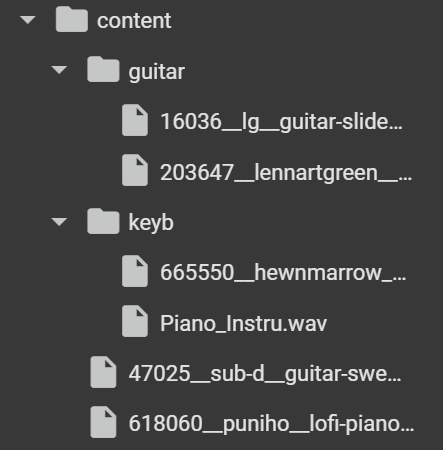
gt_files = os.listdir('/content/guitar/')
kb_files = os.listdir('/content/keyb/')

gt_files = [f for f in gt_files if os.path.isfile(os.path.join('/content/guitar/', f))]
kb_files = [f for f in kb_files if os.path.isfile(os.path.join('/content/keyb/', f))]

# แปลงเสียงกีตาร์เป็น Spectrogram และเก็บในตัวแปร
for f in tqdm(gt_files):
    file1 = 'guitar/' + f
    data = spect(file1)
    x.append(data)
    y.append([0, 1])  # กีตาร์ = [0, 1]

# แปลงเสียงคีย์บอร์ดเป็น Spectrogram และเก็บในตัวแปร
for f in tqdm(kb_files):
    file1 = 'keyb/' + f
    data = spect(file1)
    x.append(data)
    y.append([1, 0])  # คีย์บอร์ด = [1, 0]

ขั้นตอนที่ 2: การฝึกโมเดลด้วย Convolutional Neural Networks (CNN)

ในขั้นตอนนี้เราจะนำเข้า sklearn สำหรับการสร้างชุดฝึกโมเดล tensorflow สำหรับการคำนวณสร้าง deeplearning และนำข้อมูลที่เตรียมไว้มาใช้ในการฝึกโมเดล CNN ซึ่งมีการใช้ Conv2D เพื่อการเรียนรู้ฟีเจอร์จาก Spectrogram ในการประมวลภาพ และ MaxPooling2D เพื่อลดขนาดข้อมูล พร้อมทั้งใช้ Dense และ Flatten เพื่อให้สามารถจำแนกประเภทเสียงได้

from sklearn.model_selection import train_test_split
import tensorflow as tf
from keras.models import Sequential
from keras.layers import Conv2D, MaxPooling2D, Dense, Flatten
from keras.optimizers import RMSprop

# แบ่งข้อมูลเป็น training และ testing
x = np.array(x)
y = np.array(y)
x = x.reshape(x.shape[0], x.shape[1], x.shape[2], 1)

xtrain, xtest, ytrain, ytest = train_test_split(x, y, train_size=0.8, random_state=42)

# สร้างโมเดล CNN
model = Sequential([
    Conv2D(128, (3, 3), activation='relu', input_shape=xtrain.shape[1:]),
    MaxPooling2D(pool_size=(2, 2)),
    Conv2D(128, (3, 3), activation='relu'),
    MaxPooling2D(pool_size=(2, 2)),
    Dense(16),
    Dense(8),
    Flatten(),
    Dense(2, activation='softmax')
])

# คอมไพล์โมเดล หรือการเตรียมโมเดลสำหรับการฝึกฝน
model.compile(optimizer=RMSprop(learning_rate=0.0001), loss='categorical_crossentropy', metrics=['accuracy'])

# ฝึกฝนโมเดล 100 รอบ
history = model.fit(xtrain, ytrain, epochs=100, validation_data=(xtest, ytest))

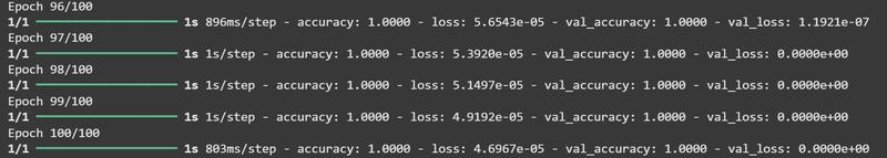
จากผลลัพธ์การ train ครบ 100 ครั้ง
ผลการ train ครั้งที่ 100 พบว่าตัวโมเดลมี ความแม่นยำสูงในการฝึก (accuracy: 1.0000) และค่าความสูญเสียต่ำในข้อมูลการฝึก (loss: 4.6967e-05) ซึ่งบ่งชี้ว่าโมเดลสามารถจำแนกประเภทของข้อมูลในชุดการฝึกได้ดี แต่ในขณะเดียวกัน, โมเดลไม่สามารถทำนายผลได้ดีในข้อมูลทดสอบ (val_accuracy: 1.0000) และค่าความสูญเสียต่ำมาก (val_loss: 0.0000) ซึ่งแสดงถึงผลที่ดีในการทดสอบ.

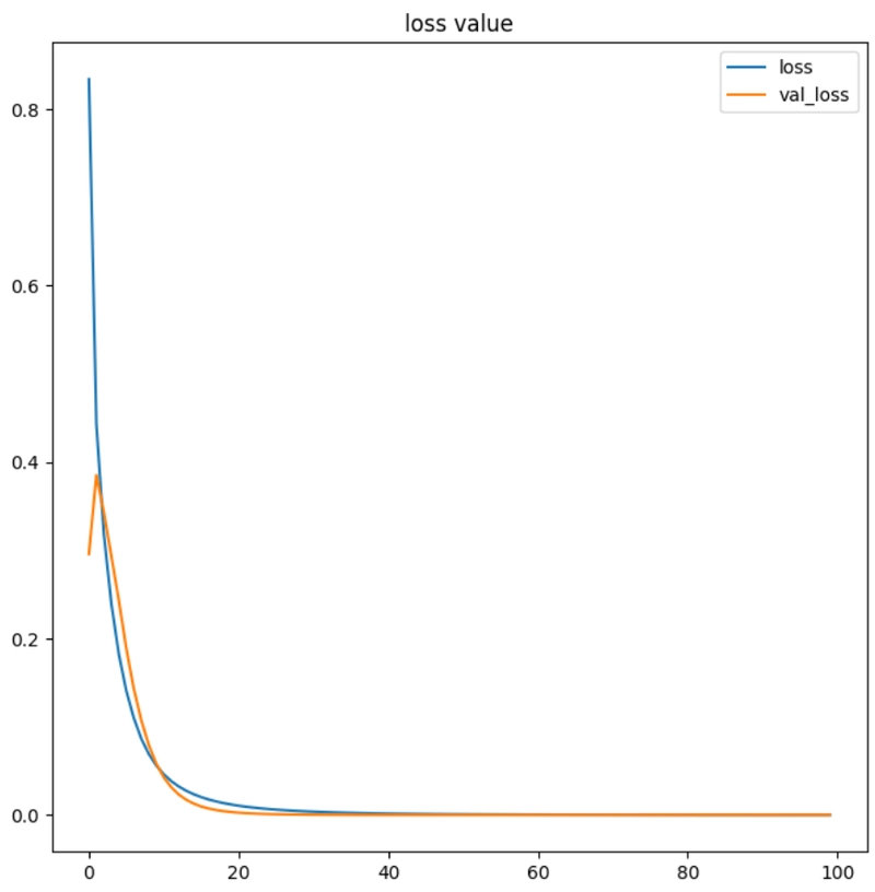
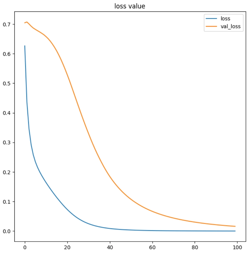
ต่อมาจะใช้ matplotlib เพื่อวาดกราฟที่แสดงถึง ค่า loss และ accuracy ของโมเดลที่เราได้ฝึกในแต่ละรอบ

plt.figure(figsize=(8,8))
plt.title('loss value')
plt.plot(history.history['loss'])
plt.plot(history.history['val_loss'])
plt.legend(['loss', 'val_loss'])
print('los:', history.history['loss'][-1])
print('val_loss:', history.history['val_loss'][-1])
plt.show()
plt.figure(figsize=(8,8))
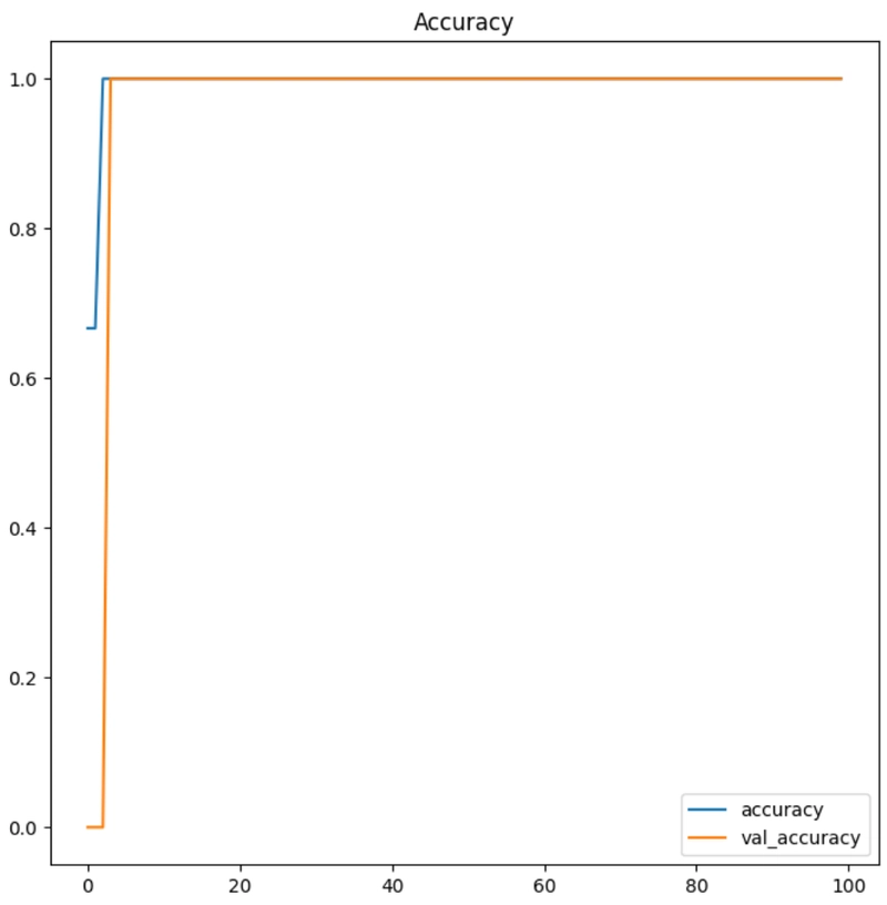
plt.title('Accuracy')
plt.plot(history.history['accuracy'])
plt.plot(history.history['val_accuracy'])
plt.legend(['accuracy', 'val_accuracy'])
print('acc:', history.history['accuracy'][-1])
print('val_acc:', history.history['val_accuracy'][-1])
plt.show()

los: 4.6966906666057184e-05 val_loss: 0.0

acc: 1.0 val_acc: 1.0

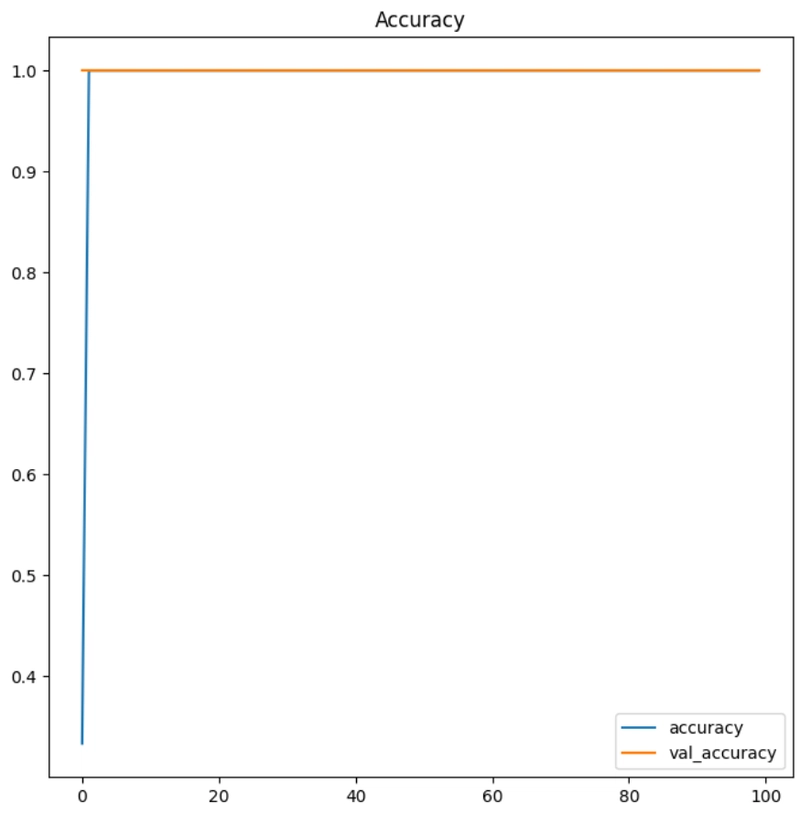
จากผลลัพธ์ แสดงให้เห็นว่าในช่วงการฝึก (Training) โมเดลมีความแม่นยำสูงในการฝึก (accuracy: 1.0000) และ ค่าความสูญเสียต่ำในข้อมูลการฝึก (loss: 4.6967e-05) และในขณะเดียวกัน มีความแม่นยำสูงในข้อมูลทดสอบ (val_accuracy: 1.0000) และ ค่าความสูญเสียเป็น 0 ในข้อมูลทดสอบ (val_loss: 0.0) ซึ่งบ่งชี้ว่าโมเดลสามารถเรียนรู้ได้ดีทั้งในข้อมูลการฝึกและข้อมูลทดสอบ

ซึ่งการเรียนรู้ของโมเดลนั้นจะขึ้นอยู่กับข้อมูล Audio ที่นำมาเทรน หากเป็นเสียงที่ต่างกันมากก็จะมี accuracy มาก หากเป็นเสียงที่คล้ายกันมากก็อาจทำให้ accuracy ลดลง

ขั้นตอนที่ 3: การประเมินผลและทดลองใช้

หลังจากฝึกฝนโมเดลแล้ว, เราสามารถนำโมเดลไปใช้ในการทำนายประเภทของเสียงจากไฟล์เสียงอื่นๆ ในที่นี้คือไฟล์เสียงที่เราเตรียมไว้สำหรับการ test โดยใช้ฟังก์ชัน wav2predict() ที่จะทำการแปลงเสียงเป็น Spectrogram และทำนายว่าเป็นเสียงของ กีตาร์ หรือ คีย์บอร์ด

def wav2predict(sf):
    data = spect(sf)
    data2arr = np.array(data)
    testsound = data2arr.reshape(1, data2arr.shape[0], data2arr.shape[1], 1)
    p = model.predict(testsound)
    label = ['keyboard', 'guitar']
    i = np.argmax(p)
    prop = np.max(p)
    result = label[i]
    return result, prop

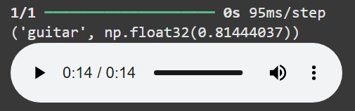
music = '/content/47025__sub-d__guitar-swell-5.wav'
r = wav2predict(music)
print (r)
Audio(music)

music = '/content/618060__puniho__lofi-piano-loop-15-80bpm.wav'
r = wav2predict(music)
print (r)
Audio(music)

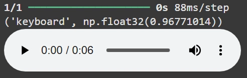
ซึ่งโมเดลตัวนี้ก็สามารถบอกได้อย่างถูกต้องว่าอันไหนคือเสียงเปียโนและอันไหนคือเสียงกีต้าร์

ตัวอย่างเพิ่มเติม

คราวนี้จะลองให้ตัวโมเดลแยกเสียงสัตว์ดูบ้าง ระหว่างเสียงนก และแมว
โดยจะมีเสียงนก และแมวที่เอาไว้ train โฟลเดอร์ละ 2 เสียง และเสียงที่เอาไว้ test อีกอย่างละ 1 เสียง

ขั้นตอนที่ 1: การเตรียมข้อมูลสำหรับโมเดล

เใช้การตรียมข้อมูลเหมือนเดิมแต่เปลี่ยน ชื่อไฟล์, ตัวแปร และโฟลเดอร์ให้ถูกต้อง

import librosa, librosa.display
import numpy as np
import matplotlib.pyplot as plt
from IPython.display import Audio
import os
from tqdm import tqdm
import warnings

def spect(wave):
    f, sr = librosa.load(wave, duration=0.9)
    st = librosa.stft(f)
    spectrogram = np.abs(st)
    return spectrogram

x = list()
y = list()

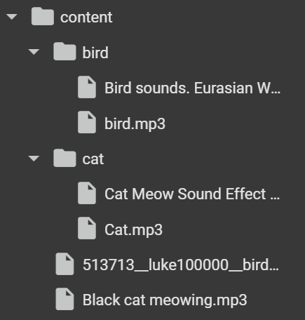
# อ่านไฟล์เสียงจากโฟลเดอร์ต่าง ๆ
cat_files = os.listdir('/content/cat/')
bird_files = os.listdir('/content/bird/')

cat_files = [f for f in cat_files if os.path.isfile(os.path.join('/content/cat/', f))]
bird_files = [f for f in bird_files if os.path.isfile(os.path.join('/content/bird/', f))]

# แปลงเสียงกีตาร์เป็น Spectrogram และเก็บในตัวแปร
for f in tqdm(cat_files):
    file1 = 'cat/' + f
    data = spect(file1)
    x.append(data)
    y.append([0, 1])  # แมว = [0, 1]

# แปลงเสียงคีย์บอร์ดเป็น Spectrogram และเก็บในตัวแปร
for f in tqdm(bird_files):
    file1 = 'bird/' + f
    data = spect(file1)
    x.append(data)
    y.append([1, 0])  # นก = [1, 0]

ขั้นตอนที่ 2: การฝึกโมเดลด้วย Convolutional Neural Networks (CNN)

นำโมเดลมา train ด้วยวิธีเดิม

from sklearn.model_selection import train_test_split
import tensorflow as tf
from keras.models import Sequential
from keras.layers import Conv2D, MaxPooling2D, Dense, Flatten
from keras.optimizers import RMSprop

# แบ่งข้อมูลเป็น training และ testing
x = np.array(x)
y = np.array(y)
x = x.reshape(x.shape[0], x.shape[1], x.shape[2], 1)

xtrain, xtest, ytrain, ytest = train_test_split(x, y, train_size=0.8, random_state=42)

# สร้างโมเดล CNN
model = Sequential([
    Conv2D(128, (3, 3), activation='relu', input_shape=xtrain.shape[1:]),
    MaxPooling2D(pool_size=(2, 2)),
    Conv2D(128, (3, 3), activation='relu'),
    MaxPooling2D(pool_size=(2, 2)),
    Dense(16),
    Dense(8),
    Flatten(),
    Dense(2, activation='softmax')
])

# คอมไพล์โมเดล หรือการเตรียมโมเดลสำหรับการฝึกฝน
model.compile(optimizer=RMSprop(learning_rate=0.0001), loss='categorical_crossentropy', metrics=['accuracy'])

# ฝึกฝนโมเดล 100 รอบ
history = model.fit(xtrain, ytrain, epochs=100, validation_data=(xtest, ytest))

*จากผลลัพธ์การ train ครบ 100 ครั้ง *
ผลการ train ครั้งที่ 100 โมเดลมี ความแม่นยำสูง ในการฝึก (accuracy: 1.0000) และ ค่าความสูญเสียต่ำ ในข้อมูลการฝึก (loss: 2.1301e-04) ในขณะที่มี ความแม่นยำสูง ในข้อมูลทดสอบ (val_accuracy: 1.0000) และ ค่าความสูญเสียต่ำ ในข้อมูลทดสอบ (val_loss: 0.0161)

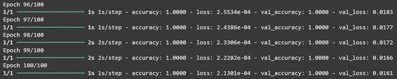
los: 0.00021300744265317917 val_loss: 0.016095701605081558

acc: 1.0 val_acc: 1.0

จากผลลัพธ์ แสดงให้เห็นว่าในช่วงการฝึก (Training) โมเดลมีความแม่นยำสูงในการฝึก (accuracy: 1.0000) และ ค่าความสูญเสียต่ำในข้อมูลการฝึก (loss: 0.00021300744265317917) ขณะเดียวกันโมเดลยังคงสามารถทำนายผลได้ดีในข้อมูลทดสอบ (val_accuracy: 1.0000) และ ค่าความสูญเสียต่ำในข้อมูลทดสอบ (val_loss: 0.016095701605081558)

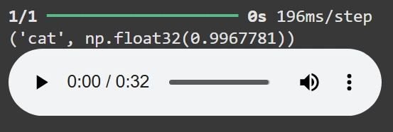
ขั้นตอนที่ 3: การประเมินผลและทดลองใช้

นำโมเดลมาลองทดสอบจำแนกเสียงจากไฟล์เสียงอื่น ๆ ในที่นี้คือไฟล์เสียงที่เราเตรียมไว้สำหรับการ test

def wav2predict(sf):
    data = spect(sf)
    data2arr = np.array(data)
    testsound = data2arr.reshape(1, data2arr.shape[0], data2arr.shape[1], 1)
    p = model.predict(testsound)
    label = ['bird', 'cat']
    i = np.argmax(p)
    prop = np.max(p)
    result = label[i]
    return result, prop

music = '/content/Tombird.mp3'
r = wav2predict(music)
print (r)
Audio(music)

music = '/content/513713__luke100000__birds-chirping.wav'
r = wav2predict(music)
print (r)
Audio(music)

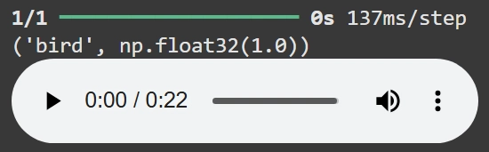
ซึ่งโมเดลตัวนี้ก็สามารถบอกได้อย่างถูกต้องว่าอันไหนคือเสียงแมมวและอันไหนคือเสียงนกเช่นเดียวกัน

สรุปผล

ในบทความนี้เราได้ใช้เทคนิค Deep Learning และ CNN ในการจำแนกเสียงจากเครื่องดนตรีคือ เสียงกีตาร์ และเสียงคีย์บอร์ดเปียใน และจำแนกเสียงสัตว์คือ เสียงนก และเสียงแมว โดยเริ่มจากการแปลงข้อมูลเสียงเป็น Spectrogram และนำข้อมูลนี้ไปฝึกโมเดลเพื่อทำนายประเภทของเสียงอื่น ๆ ซึ่งเทคนิคนี้สามารถประยุกต์ใช้ในการจำแนกประเภทเสียงอื่น ๆ ได้เช่นกัน