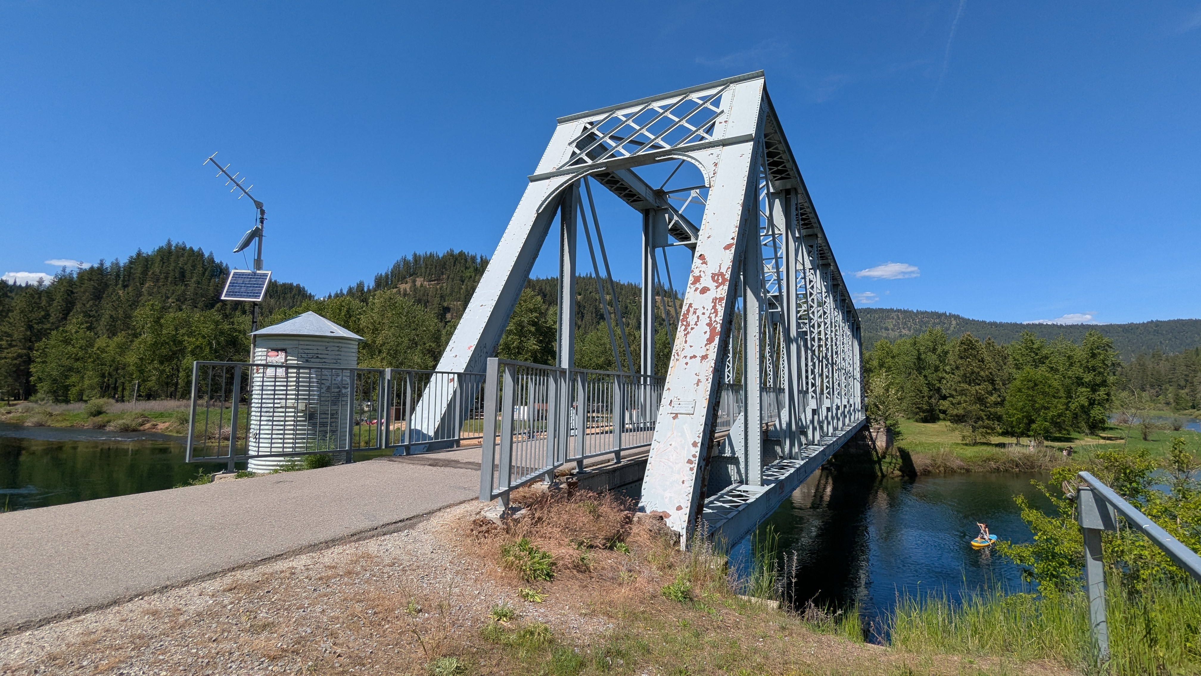
Remotely Interesting: Stream Gages

Near my childhood home was a small river. It wasn’t much more than a creek at the best of times, and in dry summers it would sometimes almost dry up …read more

May 28, 2025 - 22:40

Near my childhood home was a small river. It wasn’t much more than a creek at the best of times, and in dry summers it would sometimes almost dry up completely. But snowmelt revived it each Spring, and the remains of tropical storms in late Summer and early Fall often transformed it into a raging torrent if only briefly before the flood waters receded and the river returned to its lazy ways.

Other than to those of us who used it as a playground, the river seemed of little consequence. But it did matter enough that a mile or so downstream was some sort of instrumentation, obviously meant to monitor the river. It was — and still is — visible from the road, a tall corrugated pipe standing next to the river, topped with a box bearing the logo of the US Geological Survey. On occasion, someone would visit and open the box to do mysterious things, which suggested the river was interesting beyond our fishing and adventuring needs.

Although I learned quite early that this device was a streamgage, and that it was part of a large network of monitoring instruments the USGS used to monitor the nation’s waterways, it wasn’t until quite recently — OK, this week — that I learned how streamgages work, or how extensive the network is. A lot of effort goes into installing and maintaining this far-flung network, and it’s worth looking at how these instruments work and their impact on everyday life.

Inventing Hydrography

First, to address the elephant in the room, “gage” is a rarely used but accepted alternative spelling of “gauge.” In general, gage tends to be used in technical contexts, which certainly seems to be the case here, as opposed to a non-technical context such as “A gauge of public opinion.” Moreover, the USGS itself uses that spelling, for interesting historical reasons that they’ve apparently had to address often enough that they wrote an FAQ on the subject. So I’ll stick with the USGS terminology in this article, even if I really don’t like it that much.

With that out of the way, the USGS has a long history of monitoring the nation’s rivers. The first streamgaging station was established in 1889 along the Rio Grande River at a railroad station in Embudo, New Mexico. Measurements were entirely manual in those days, performed by crews trained on-site in the nascent field of hydrography. Many of the tools and methods that would be used through the rest of the 19th century to measure the flow of rivers throughout the West and later the rest of the nation were invented at Embudo.

Then as now, river monitoring boils down to one critical measurement: discharge rate, or the volume of water passing a certain point in a fixed amount of time. In the US, discharge rate is measured in cubic feet per second, or cfs. The range over which discharge rate is measured can be huge, from streams that trickle a few dozen cubic feet of water every second to the over one million cfs discharge routinely measured at the mouth of the mighty Mississippi each Spring.

Measurements over such a wide dynamic range would seem to be an engineering challenge, but hydrographers have simplified the problem by cheating a little. While volumetric flow in a closed container like a pipe is relatively easy — flowmeters using paddlewheels or turbines are commonly used for such a task — direct measurement of flow rates in natural watercourses is much harder, especially in navigable rivers where such measuring instruments would pose a hazard to navigation. Instead, the USGS calculates the discharge rate indirectly using stream height, often referred to as flood stage.

Beside Still Waters

Schematic of a USGS stilling well. The water level in the well tracks the height of the stream, with a bit of lag. The height of the water column in the well is easier to read than the surface of the river. Source: USGS, public domain.

The height of a river at any given point is much easier to measure, with the bonus that the tools used for this task lend themselves to continuous measurements. Stream height is the primary data point of each streamgage in the USGS network, which uses several different techniques based on the specific requirements of each site.

A float-tape gage, with a counterweighted float attached to an encoder by a stainless steel tape. The encoder sends the height of the water column in the stilling well to the data logger. Source: USGS, public domain.

The most common is based on a stilling well. Stilling wells are vertical shafts dug into the bank adjacent to a river. The well is generally large enough for a technician to enter, and is typically lined with either concrete or steel conduit, such as the streamgage described earlier. The bottom of the shaft, which is also lined with an impervious material such as concrete, lies below the bottom of the river bed, while the height of the well is determined by the highest expected flood stage for the river. The lumen of the well is connected to the river via a pair of pipes, which terminate in the water above the surface of the riverbed. Water fills the well via these input pipes, with the level inside the well matching the level of the water in the river.

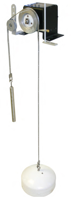
As the name implies, the stilling well performs the important job of damping any turbulence in the river, allowing for a stable column of water whose height can be easily measured. Most stilling wells measure the height of the water column with a float connected to a shaft encoder by a counterweighted stainless steel tape. Other stilling wells are measured using ultrasonic transducers, radar, or even lidar scanners located in the instrument shelter on the top of the well, which translate time-of-flight to the height of the water column.

While stilling well gages are cheap and effective, they are not without their problems. Chief among these is dealing with silt and debris. Even though intakes are placed above the bottom of the river, silt enters the stilling well and settles into the sump. This necessitates frequent maintenance, usually by flushing the sump and the intake lines using water from a flushing tank located within the stilling well. In rivers with a particularly high silt load, there may be a silt trap between the intakes and the stilling well. Essentially a concrete box with a series of vertical baffles, the silt trap allows silt to settle out of the river water before it enters the stilling well, and must be cleaned out periodically.

Bubbles, Bubbles

Bubble gages often live on pilings or other structures within the watercourse.

Making up for some of the deficiencies of the stilling well is the bubble gage, which measures river stage using gas pressure. A bubble gage typically consists of a small air pump or gas cylinders inside the instrument shelter, plumbed to a pipe that comes out below the surface of the river. As with stilling wells, the tube is fixed at a known point relative to a datum, which is the reference height for that station. The end of the pipe in the water has an orifice of known size, while the supply side has regulators and valves to control the flow of gas. River stage can be measured by sensing the gas pressure in the system, which will increase as the water column above the orifice gets higher.

Bubble gages have a distinct advantage over stilling wells in rivers with a high silt load, since the positive pressure through the orifice tends to keep silt out of the works. However, bubble gages tend to need a steady supply of electricity to power their air pump continuously, or for gages using bottled gas, frequent site visits for replenishment. Also, the pipe run to the orifice needs to be kept fairly short, meaning that bubble gage instrument shelters are often located on pilings within the river course or on bridge abutments, which can make maintenance tricky and pose a hazard to navigation.

While bubble gages and stilling wells are the two main types of gaging stations for fixed installations, the USGS also maintains a selection of temporary gaging instruments for tactical use, often for response to natural disasters. These Rapid Deployment Gages (RDGs) are compact units designed to affix to the rail of a bridge or some other structure across the river. Most RDGs use radar to sense the water level, but some use sonar.

Go With the Flow

No matter what method is used to determine the stage of a river, calculating the discharge rate is the next step. To do that, hydrographers have to head to the field and make flow measurements. By measuring the flow rates at intervals across the river, preferably as close as possible to the gaging station, the total flow through the channel at that point can be estimated, and a calibration curve relating flow rate to stage can be developed. The discharge rate can then be estimated from just the stage reading.

Flow readings are taken using a variety of tools, depending on the size of the river and the speed of the current. Current meters with bucket wheels can be lowered into a river on a pole; the flow rotates the bucket wheel and closes electrical contacts that can be counted on an electromagnetic totalizer. More recently, Acoustic Doppler Current Profilers (ADCPs) have come into use. These use ultrasound to measure the velocity of particulates in the water by their Doppler shift.

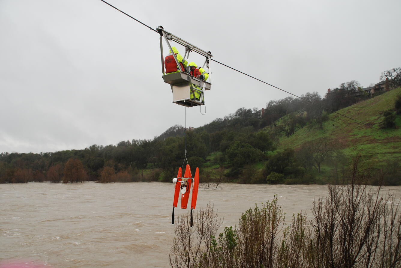
Crews can survey the entire width of a small stream by wading, from boats, or by making measurements from a convenient bridge. In some remote locations where the river is especially swift, the USGS may erect a cableway across the river, so that measurements can be taken at intervals from a cable car.

Nice work if you can get it. USGS crew making flow measurements from a cableway over the American River in California using an Acoustic Doppler Current Profiler. Source: USGS, public domain.

From Paper to Satellites

In the earliest days of streamgaging, recording data was strictly a pen-on-paper process. Station log books were updated by hydrographers for every observation, with results transmitted by mail or telegraph. Later, stations were equipped with paper chart recorders using a long-duration clockwork mechanism. The pen on the chart recorder was mechanically linked to the float in a stilling well, deflecting it as the river stage changed and leaving a record on the chart. Electrical chart recorders came next, with the position of the pen changing based on the voltage through a potentiometer linked to the float.

Chart recorders, while reliable, have the twin disadvantages of needing a site visit to retrieve the data and requiring a tedious manual transcription of the chart data to tabular form. To solve the latter problem, analog-digital recorders (ADRs) were introduced in the 1960s. These recorded stage data on paper tape as four binary-coded decimal (BCD) digits. The time of each stage reading was inferred from its position on the tape, given a known starting time and reading interval. Tapes still had to be retrieved from each station, but at least reading the data back at the office could be automated with a paper tape reader.

In the 1980s and 1990s, gaging stations were upgraded to electronic data loggers, with small solar panels and batteries where grid power wasn’t available. Data was stored locally in the logger between maintenance visits by a hydrographer, who would download the data. Alternately, gaging stations located close to public rights of way sometimes had leased telephone lines for transmitting data at intervals via modem. Later, gaging stations started sprouting cross-polarized Yagi antennas, aimed at one of the Geostationary Operational Environmental Satellites (GOES). Initially, gaging stations used one of the GOES low data rate telemetry channels with a 100 to 300 bps connection. This gave hydrologists near-real-time access to gaging data for the first time. Since 2013, all stations have been upgraded to a high data rate channel that allows up to 1,200 bps telemetry.

Currently, gage data is collected every 15 minutes normally, although the interval can be increased to every 5 minutes at times of peak flow. Data is buffered locally before a GOES uplink, which is about every hour or so, or as often as every 15 minutes in peak flow or emergencies. The uplink frequencies and intervals are very well documented on the USGS site, so you can easily pick them up with an SDR, and you can see if the creek is rising from the comfort of your own shack.