




![[The AI Show Episode 146]: Rise of “AI-First” Companies, AI Job Disruption, GPT-4o Update Gets Rolled Back, How Big Consulting Firms Use AI, and Meta AI App](https://www.marketingaiinstitute.com/hubfs/ep%20146%20cover.png)


![Life in Startup Pivot Hell with Ex-Microsoft Lonewolf Engineer Sam Crombie [Podcast #171]](https://cdn.hashnode.com/res/hashnode/image/upload/v1746753508177/0cd57f66-fdb0-4972-b285-1443a7db39fc.png?#)


.png?width=1920&height=1920&fit=bounds&quality=70&format=jpg&auto=webp#)


.png?width=1920&height=1920&fit=bounds&quality=70&format=jpg&auto=webp#)


_Aleksey_Funtap_Alamy.jpg?width=1280&auto=webp&quality=80&disable=upscale#)
_Sergey_Tarasov_Alamy.jpg?width=1280&auto=webp&quality=80&disable=upscale#)


![Apple Foldable iPhone to Feature New Display Tech, 19% Thinner Panel [Rumor]](https://www.iclarified.com/images/news/97271/97271/97271-640.jpg)
![Apple Developing New Chips for Smart Glasses, Macs, AI Servers [Report]](https://www.iclarified.com/images/news/97269/97269/97269-640.jpg)
![Apple Shares New Mother's Day Ad: 'A Gift for Mom' [Video]](https://www.iclarified.com/images/news/97267/97267/97267-640.jpg)
![Apple Shares Official Trailer for 'Stick' Starring Owen Wilson [Video]](https://www.iclarified.com/images/news/97264/97264/97264-640.jpg)


Model Compression: Make Your Machine Learning Models Lighter and Faster
A deep dive into pruning, quantization, distillation, and other techniques to make your neural networks more efficient and easier to deploy. The post Model Compression: Make Your Machine Learning Models Lighter and Faster appeared first on Towards Data Science.

Introduction
Whether you’re preparing for interviews or building Machine Learning systems at your job, model compression has become a must-have skill. In the era of LLMs, where models are getting larger and larger, the challenges around compressing these models to make them more efficient, smaller, and usable on lightweight machines have never been more relevant.
In this article, I will go through four fundamental compression techniques that every ML practitioner should understand and master. I explore pruning, quantization, low-rank factorization, and Knowledge Distillation, each offering unique advantages. I will also add some minimal PyTorch code samples for each of these methods.
I hope you enjoy the article!
- Feel free to connect on LinkedIn!
- Follow me on GitHub and visit my website for more content.
Model pruning
Pruning is probably the most intuitive compression technique. The idea is very simple: remove some of the weights of the network, either randomly or remove the “less important” ones. Of course, when we talk about “removing” weights in the context of neural networks, it means setting the weights to zero.

Structured vs unstructured pruning
Let’s start with a simple heuristic: removing weights smaller than a threshold.
\[ w’_{ij} = \begin{cases} w_{ij} & \text{if } |w_{ij}| \ge \theta_0 \\
0 & \text{if } |w_{ij}| < \theta_0
\end{cases} \]
Of course, this is not ideal because we would need to find a way to find the right threshold for our problem! A more practical approach is to remove a specified proportion of weights with the smallest magnitudes (norm) within one layer. There are 2 common ways of implementing pruning in one layer:
- Structured pruning: remove entire components of the network (e.g. a random row from the weight tensor, or a random channel in a convulational layer)
- Unstructured pruning: remove individual weights regardless of their positions and of the structure of the tensor
We can also use global pruning with either of the two above methods. This will remove the chosen proportion of weights across multiple layers, and potentially have different removal rates depending on the number of parameters in each layer.
PyTorch makes this pretty straightforward (by the way, you can find all code snippets in my GitHub repo).
import torch.nn.utils.prune as prune

# 1. Random unstructured pruning (20% of weights at random)
prune.random_unstructured(model.layer, name="weight", amount=0.2)

# 2. L1‑norm unstructured pruning (20% of smallest weights)
prune.l1_unstructured(model.layer, name="weight", amount=0.2)

# 3. Global unstructured pruning (40% of all weights by L1 norm across layers)
prune.global_unstructured(
    [(model.layer1, "weight"), (model.layer2, "weight")],
    pruning_method=prune.L1Unstructured,
    amount=0.4
)

# 4. Structured pruning (remove 30% of rows with lowest L2 norm)
prune.ln_structured(model.layer, name="weight", amount=0.3, n=2, dim=0)
Note: if you have taken statistics classes, you probably learned regularization-induced methods that also implicitly prune some weights during training, by using L0 or L1 norm regularization. Pruning differs from that because it is applied as a post-Model Compression technique
Why does pruning work? The Lottery Ticket Hypothesis

I would like to conclude that section with a quick mention of the Lottery Ticket Hypothesis, which is both an application of pruning and an interesting explanation of how removing weights can often improve a model. I recommend reading the associated paper ([7]) for more details.
Authors use the following procedure:
- Train the full model to convergence
- Prune the smallest-magnitude weights (say 10%)
- Reset the remaining weights to their original initialization values
- Retrain this pruned network
- Repeat the process multiple times
After doing this 30 times, you end up with only 0.930 ~ 4% of the original parameters. And surprisingly, this network can do as well as the original one.
This suggests that there is important parameter redundancy. In other words, there exists a sub-network (“a lottery ticket”) that actually does most of the work!
Pruning is one way to unveil this sub-network.
I recommend this very good video that covers the topic!
Quantization
While pruning focuses on removing parameters entirely, Quantization takes a different approach: reducing the precision of each parameter.
Remember that every number in a computer is stored as a sequence of bits. A float32 value uses 32 bits (see example picture below), whereas an 8-bit integer (int8) uses just 8 bits.

Most deep learning models are trained using 32-bit floating-point numbers (FP32). Quantization converts these high-precision values to lower-precision formats like 16-bit floating-point (FP16), 8-bit integers (INT8), or even 4-bit representations.
The savings here are obvious: INT8 requires 75% less memory than FP32. But how do we actually perform this conversion without destroying our model’s performance?
The math behind quantization
To convert from floating-point to integer representation, we need to map the continuous range of values to a discrete set of integers. For INT8 quantization, we’re mapping to 256 possible values (from -128 to 127).
Suppose our weights are normalized between -1.0 and 1.0 (common in deep learning):
\[ \text{scale} = \frac{\text{float_max} – \text{float_min}}{\text{int8_max} – \text{int8_min}} = \frac{1.0 – (-1.0)}{127 – (-128)} = \frac{2.0}{255} \]
Then, the quantized value is given by
\[\text{quantized_value} = \text{round}(\frac{\text{original_value}}{\text{scale}} \] + \text{zero_point})
Here, zero_point=0 because we want 0 to be mapped to 0. We can then round this value to the nearest integer to get integers between -127 and 128.
And, you guessed it: to get integers back to float, we can use the inverse operation: \[\text{float_value} = \text{integer_value} \times \text{scale} – \text{zero_point} \]
Note: in practice, the scaling factor is determined based on the range values we quantize.
How to apply quantization?
Quantization can be applied at different stages and with different strategies. Here are a few techniques worth knowing about: (below, the word “activation” refers to the output values of each layer)
- Post-training quantization (PTQ):
- Static Quantization: quantize both weights and activations offline (after training and before inference)
- Dynamic Quantization: quantize weights offline, but activations on-the-fly during inference. This is different from offline quantization because the scaling factor is determined based on the values seen so far during inference.
- Quantize-aware training (QAT): simulate quantization during training by rounding values, but calculations are still done with floating-point numbers. This makes the model learn weights that are more robust to quantization, which will be applied after training. Under the hood, the idea is to add “fake” operations:
x -> dequantize(quantize(x)): this new value is close to x, but it still helps the model tolerate the 8-bit rounding and clipping noise.
import torch.quantization as tq

# 1. Post‑training static quantization (weights + activations offline)
model.eval()
model.qconfig = tq.get_default_qconfig('fbgemm') # assign a static quantization config
tq.prepare(model, inplace=True)
# we need to use a calibration dataset to determine the ranges of values
with torch.no_grad():
    for data, _ in calibration_data:
        model(data)
tq.convert(model, inplace=True) # convert to a fully int8 model

# 2. Post‑training dynamic quantization (weights offline, activations on‑the‑fly)
dynamic_model = tq.quantize_dynamic(
    model,
    {torch.nn.Linear, torch.nn.LSTM}, # layers to quantize
    dtype=torch.qint8
)

# 3. Quantization‑Aware Training (QAT)
model.train()
model.qconfig = tq.get_default_qat_qconfig('fbgemm')  # set up QAT config
tq.prepare_qat(model, inplace=True) # insert fake‑quant modules
# [here, train or fine‑tune the model as usual]
qat_model = tq.convert(model.eval(), inplace=False) # convert to real int8 after QAT
Quantization is very flexible! You can apply different precision levels to different parts of the model. For instance, you might quantize most linear layers to 8-bit for maximum speed and memory savings, while leaving critical components (e.g. attention heads, or batch-norm layers) at 16-bit or full-precision.
Low-Rank Factorization
Now let’s talk about low-rank factorization — a method that has been popularized with the rise of LLMs.
The key observation: many weight matrices in neural networks have effective ranks much lower than their dimensions suggest. In plain English, that means there is a lot of redundancy in the parameters.
Note: if you have ever used PCA for dimensionality reduction, you have already encountered a form of low-rank approximation. PCA decomposes large matrices into products of smaller, lower-rank factors that retain as much information as possible.
The linear algebra behind low-rank factorization
Take a weight matrix W. Every real matrix can be represented using a Singular Value Decomposition (SVD):
\[ W = U\Sigma V^T \]
where Σ is a diagonal matrix with singular values in non-increasing order. The number of positive coefficients actually corresponds to the rank of the matrix W.

To approximate W with a matrix of rank k < r, we can select the k greatest elements of sigma, and the corresponding first k columns and first k rows of U and V respectively:
\[ \begin{aligned} W_k &= U_k\,\Sigma_k\,V_k^T
\\[6pt] &= \underbrace{U_k\,\Sigma_k^{1/2}}_{A\in\mathbb{R}^{m\times k}} \underbrace{\Sigma_k^{1/2}\,V_k^T}_{B\in\mathbb{R}^{k\times n}}. \end{aligned} \]
See how the new matrix can be decomposed as the product of A and B, with the total number of parameters now being m * k + k * n = k*(m+n) instead of m*n! This is a huge improvement, especially when k is much smaller than m and n.
In practice, it’s equivalent to replacing a linear layer x → Wx with 2 consecutive ones: x → A(Bx).
In PyTorch
We can either apply low-rank factorization before training (parameterizing each linear layer as two smaller matrices – not really a compression method, but a design choice) or after training (applying a truncated SVD on weight matrices). The second approach is by far the most common one and is implemented below.
import torch

# 1. Extract weight and choose rank
W = model.layer.weight.data # (m, n)
k = 64 # desired rank

# 2. Approximate low-rank SVD
U, S, V = torch.svd_lowrank(W, q=k) # U: (m, k), S: (k, k), V: (n, k)

# 3. Form factors A and B
A = U * S.sqrt() # [m, k]
B = V.t() * S.sqrt().unsqueeze(1) # [k, n]

# 4. Replace with two linear layers and insert the matrices A and B
orig = model.layer
model.layer = torch.nn.Sequential(
    torch.nn.Linear(orig.in_features, k, bias=False),
    torch.nn.Linear(k, orig.out_features, bias=False),
)
model.layer[0].weight.data.copy_(B)
model.layer[1].weight.data.copy_(A)
LoRA: an application of low-rank approximation

I think it’s crucial to mention LoRA: you have probably heard of LoRA (Low-Rank Adaptation) if you have been following LLM fine-tuning developments. Though not strictly a compression technique, LoRA has become extremely popular for efficiently adapting large language models and making fine-tuning very efficient.
The idea is simple: during fine-tuning, rather than modifying the original model weights W, LoRA freezes them and learn trainable low-rank updates:
$$W’ = W + \Delta W = W + AB$$
where A and B are low-rank matrices. This allows for task-specific adaptation with just a fraction of the parameters.
Even better: QLoRA takes this further by combining quantization with low-rank adaptation!
Again, this is a very flexible technique and can be applied at various stages. Usually, LoRA is applied only on specific layers (for example, Attention layers’ weights).
Knowledge Distillation

Knowledge distillation takes a fundamentally different approach from what we have seen so far. Instead of modifying an existing model’s parameters, it transfers the “knowledge” from a large, complex model (the “teacher”) to a smaller, more efficient model (the “student”). The goal is to train the student model to mimic the behavior and replicate the performance of the teacher, often an easier task than solving the original problem from scratch.
The distillation loss
Let’s explain some concepts in the case of a classification problem:
- The teacher model is usually a large, complex model that achieves high performance on the task at hand
- The student model is a second, smaller model with a different architecture, but tailored to the same task
- Soft targets: these are the teacher’s model predictions (probabilities, and not labels!). They will be used by the student model to mimic the teacher’s behaviors. Note that we use raw predictions and not labels because they also contain information about the confidence of the predictions
- Temperature: in addition to the teacher’s prediction, we also use a coefficient T (called temperature) in the softmax function to extract more information from the soft targets. Increasing T softens the distribution and helps the student model give more importance to wrong predictions.
In practice, it is pretty straightforward to train the student model. We combine the usual loss (standard cross-entropy loss based on hard labels) with the “distillation” loss (based on the teacher’s soft targets):
$$ L_{\text{total}} = \alpha L_{\text{hard}} + (1 – \alpha) L_{\text{distill}} $$
The distillation loss is nothing but the KL divergence between the teacher and student distribution (you can see it as a measure of the distance between the 2 distributions).
$$ L_{\text{distill}} = D{KL}(q_{\text{teacher}} | | q_{\text{student}}) = \sum_i q_{\text{teacher}, i} \log \left( \frac{q_{\text{teacher}, i}}{q_{\text{student}, i}} \right) $$
As for the other methods, it is possible and encouraged to adapt this framework depending on the use case: for example, one can also compare logits and activations from intermediate layers in the network between the student and teacher model, instead of only comparing the final outputs.
Knowledge distillation in practice
Similar to the previous techniques, there are two options:
- Offline distillation: the pre-trained teacher model is fixed, and a separate student model is trained to mimic it. Both models are completely separate, and the teacher’s weights remain frozen during the distillation process.
- Online distillation: both models are trained simultaneously, with knowledge transfer happening during the joint training process.
And below, an easy way to apply offline distillation (the last code block of this article  Read More


