Learn to Build a Multilayer Perceptron with Real-Life Examples and Python Code

The perceptron is a fundamental concept in deep learning, with many algorithms stemming from its original design. In this tutorial, I’ll show you how to build both single layer and multi-layer perceptrons (MLPs) across three frameworks: Custom class...

May 31, 2025 - 03:30

Learn to Build a Multilayer Perceptron with Real-Life Examples and Python Code

The perceptron is a fundamental concept in deep learning, with many algorithms stemming from its original design.

In this tutorial, I’ll show you how to build both single layer and multi-layer perceptrons (MLPs) across three frameworks:

Custom classifier
Scikit-learn’s MLPClassifier
Keras Sequential classifier using SGD and Adam optimizers.

This will help you learn about their various use cases and how they work.

Prerequisites

Mathematics (Calculus, Linear Algebra, Statistics)
Coding in Python
Basic understanding of Machine Learning concepts

What is a Perceptron?

A perceptron is one of the simplest types of artificial neurons used in Machine Learning. It’s a building block of artificial neural networks that learns from labeled data to perform classification and pattern recognition tasks, typically on linearly separable data.

A single-layer perceptron consists of a single layer of artificial neurons, called perceptrons.

But when you connect many perceptrons together in layers, you have a multi-layer perceptron (MLP). This lets the network learn more complex patterns by combining simple decisions from each perceptron. And this makes MLPs powerful tools for tasks like image recognition and natural language processing.

The perceptron consists of four main parts:

Input layer: Takes the initial numerical values into the system for further processing.
Weights: Combines input values with weights (and bias terms).
Activation function: Determines whether the neuron should fire based on the threshold value.
Output layer: Produces classification result.

Image: Organization of a perceptron. Source: Rosenblatt 1958

It performs a weighted sum of inputs, adds a bias, and passes the result through an activation function – just like logistic regression. It’s sort of like a little decision-maker that says “yes” or “no” based on the information it gets.

So for instance, when we use a sigmoid activation, its output is a probability between 0 and 1, mimicking the behavior of logistic regression.

Applications of Perceptrons

Perceptrons are applied to tasks such as:

Image classification: Perceptrons classify images containing specific objects. They achieve this by performing binary classification tasks.
Linear regression: Perceptrons can predict continuous outputs based on input features. This makes them useful for solving linear regression problems.

How the Activation Function Works

For a single perceptron used for binary classification, the most common activation function is the step function (also known as the threshold function):

$$\phi(z) = \begin{cases} 1 &\text{if } z \geq \theta \\ \\ 0 &\text{if } z < \theta \end{cases}$$

where:

ϕ(z): the output of the activation function.
z: the weighted sum of the inputs plus the bias:

$$z = \sum_{i=1}^m w_i x_i + b$$

(xi: input values, w: weight associated with each input, b: bias terms)

θ is the threshold. Often, the threshold θ is set to zero, and the bias (b) effectively controls the activation threshold.

In that case, the formula becomes:

$$\phi(z) = \begin{cases} 1 &\text{if } z \geq 0 \\ \\ 0 &\text{if } z < 0 \end{cases}$$

Image: Step Function (Author)

When the step function ϕ(z) outputs one, it signifies that the input belongs to the class labeled one.

This occurs when the weighted sum is greater than zero, leading the perceptron to predict the input is in this binary class.

While the step function is conceptually the original activation for a perceptron, its discontinuity at zero causes computational challenges.

In modern implementations, we can use other activation functions like the sigmoid function:

$$\sigma (z) = \frac {1} {1 + e^{-z}}$$

The sigmoid function also outputs zero or one depending on the weighted sum (z).

How the Loss Function Works

The loss function is a crucial concept in machine learning that quantifies the error or discrepancy between the model's predictions and the actual target values.

Its purpose is to penalize the model for making incorrect or inaccurate predictions, which guides the learning algorithm (for example, gradient descent) to adjust the model's parameters in a way that minimizes this error and improves performance.

In a binary classification task, the model may adopt the hinge loss function to penalize misclassifications by incurring an additional cost for incorrect predictions:

$$L(y, h(x)) = max(0, 1- y*h(x))$$

(h(x): prediction label, y: true label)

How to Build a Single-Layered Classifier

Now, let’s build a simple single-layer perceptron for binary classification.

1. Custom Classifier

Initialize the classifier

We’ll first initialize the classifier with weights, bias, number of epochs (n_iterations), and learning_rates.

def __init__(self, learning_rate=0.01, n_iterations=1000):
    self.learning_rate = learning_rate
    self.n_iterations = n_iterations
    self.weights = None
    self.bias = None

Define the activation function

Use a step function that returns zero if input (x) ≤ 0, else 1. By default, the threshold is set to zero.

def _step_function(self, x, threshold: int = 0):
     return np.where(x > threshold, 1, 0)

Train the model

Now it’s time to start training. The learning process involves iteratively updating the perceptron’s internal parameters: weights and bias.

This process is controlled by a specified number of training epochs defined by n_iterations.

In each epoch, the model processes the entire input dataset (X) and adjusts its weights and bias based on the difference between its predictions and the true labels (y), guided by a predefined learning_rate.

def fit(self, X, y):
    n_samples, n_features = X.shape

    self.weights = np.zeros(n_features)
    self.bias = 0

    for _ in range(self.n_iterations):
        for i in range(n_samples):
            # compute weighted sum (z)
            z = np.dot(X[i], self.weights) + self.bias

            # apply the activation function
            y_pred = self._step_function(z)

            # update weights and bias
            self.weights += self.learning_rate * (y[i] - y_pred) * X[i]
            self.bias += self.learning_rate * (y[i] - y_pred)

How the weights work in the iteration loop

The weights in a perceptron define the orientation (slope) of the decision boundary that separates the classes.

Its iterative update in the for loop aims to reduce classification errors such that:

$$\begin {align*} w_j &:= w_j + \Delta w_j \\ & := w_j + \eta (y_i - \hat y_i)x_{ij} \\ &= \begin{cases} w_j &\text{(a) } y_i - \hat y_i = 0\\ w_j + \eta x_ij &\text{(b) } y_i - \hat y_i = 1 \\ w_j - \eta x_ij &\text{(c) } y_i - \hat y_i = -1 \\ \end{cases} \end{align*}$$

(w_j: j-th weight, η: learning rate, (yi−y^i): error)

This means that:

When the prediction is correct, the error is zero, so the weight is unchanged.
When the prediction is too low (yi=1 and y^i=0), the weight is adjusted to the same direction to increase the weighted sum.
When the prediction is too high (yi=0 and y^i=1), the weight is adjusted to the opposite direction to pull the weighted sum lower.

How the bias terms work in the iteration loop

The bias determines the decision boundary’s intercept (position from the origin).

Similar to weights, we adjust the bias terms in each epoch to position the decision boundary:

$$\begin {align*} b &:= b + \Delta b \\ & := b + \eta (y_i - \hat y_i) \\ &= \begin{cases} b &\text{(a) } y_i - \hat y_i = 0\\ b + \eta &\text{(b) } y_i - \hat y_i = 1 \\ b - \eta &\text{(c) } y_i - \hat y_i = -1 \\ \end{cases} \end{align*}$$

This repeated adjustment aims to optimize the model’s ability to correctly classify the training data.

Make a prediction

Lastly, we add a function to generate an outcome value (zero or one) for a new, unseen data (X):

def predict(self, X):
      linear_output = np.dot(X, self.weights) + self.bias
      predictions = self._step_function(linear_output)
      return predictions

The entire classifier looks like this:

import numpy as np

class Perceptron:
    def __init__(self, learning_rate=0.01, n_iterations=1000):
        self.learning_rate = learning_rate
        self.n_iterations = n_iterations
        self.weights = None
        self.bias = None

    def _step_function(self, x, threshold: int = 0):
        return np.where(x > threshold, 1, 0)

    def fit(self, X, y):
        n_samples, n_features = X.shape
        self.weights = np.zeros(n_features)
        self.bias = 0

        for _ in range(self.n_iterations):
            for i in range(n_samples):
                linear_output = np.dot(X[i], self.weights) + self.bias
                y_pred = self._step_function(linear_output)
                self.weights += self.learning_rate * (y[i] - y_pred) * X[i]
                self.bias += self.learning_rate * (y[i] - y_pred)
        return self

    def predict(self, X):
        linear_output = np.dot(X, self.weights) + self.bias
        y_pred = self._step_function(linear_output)
        return y_pred

Simulate with synthetic datasets

First, we generated a synthetic linearly separable dataset using make_blob and computed a decision boundary, then train the classifier we created.

from sklearn.datasets import make_blobs
from sklearn.model_selection import train_test_split
import numpy as np

# create a mock dataset
X, y = make_blobs(n_features=2, centers=2, n_samples=1000, random_state=12)

# split
X_train, X_test, y_train, y_test = train_test_split(X, y, test_size=0.2, random_state=42)

# train the model
perceptron = Perceptron(learning_rate=0.1, n_iterations=1000).fit(X_train, y_train)

# make a prediction
y_pred_train = perceptron.predict(X_train)
y_pred_test = perceptron.predict(X_test)

# evaluate the results
acc_train = np.mean(y_pred_train == y_train)
acc_test = np.mean(y_pred_test == y_test)
print(f"Accuracy (Train): {acc_train:.3} \nAccuracy (Test): {acc_test:.3}")

Results

The classifier generated a clear, highly accurate linear decision boundary.

Accuracy (Train): 0.981
Accuracy (Test): 0.975

Decision boundary of single-layer perceptron (Custom classifier)

2. Leverage SckitLearn’s MCP Classifier

For our convenience, we’ll use sckit-learn’s build-in classifier ( MCPClassifier) to build a similar, yet more robust classifier:

model = MLPClassifier(
    hidden_layer_sizes=(), # intentionally set empty to create a single layer perceptron
    activation='logistic', # choosing a sigmoid function as an activation function
    solver='sgd', # choosing SGD optimizer
    max_iter=1000,
    random_state=42, 
    learning_rate='constant', 
    learning_rate_init=0.1
).fit(X_train, y_train)

y_pred_train = model.predict(X_train)
y_pred_test = model.predict(X_test)

acc_train = np.mean(y_pred_train == y_train)
acc_test = np.mean(y_pred_test == y_test)
print(f"MCPClassifier\nAccuracy (Train): {acc_train:.3} \nAccuracy (Test): {acc_test:.3}")

Results

The MCP Classifier generated a clear linear decision boundary with slightly better accuracy scores.

Accuracy (Train): 0.985
Accuracy (Test): 0.995

Decision boundary of single-layer perceptron (MCP Classifier)

Limitations of Single-Layer Perceptrons

Now, let’s talk about the key differences between the MCP Classifier and our custom single-layer perceptron.

Unlike more general neural networks, single-layer perceptrons use a step function as their activation.

Due to its discontinuity at x=0, the step function is not differentiable over its entire domain (−∞ to ∞).

This fundamental property precludes the use of gradient-based optimization algorithms such as SGD or Adam, as these methods depend on the computation of gradients, partial derivatives for the cost function.

In contrast, most neural networks employ differentiable activation functions (for example, sigmoid, ReLU) and loss functions (for example, MSE, Cross-Entropy) for effective optimization.

Other challenges of a single-layer perceptron include:

Limited to linear separability: Because they can only learn linear decision boundaries, they are unable to handle complex, non-linearly separable data.
Lack of depth: Being single-layered, they cannot learn complex hierarchical representations.
Limited optimizer options: As mentioned, their non-differentiable activation function precludes the use of major gradient-based optimizers.

So, in the next section, you’ll learn about multi-layered perceptrons to overcome the disadvantages.

What is a Multi-Layer Perceptron?

An MLP is a class of feedforward artificial neural network that consists of at least three layers of nodes:

an input layer,
one or more hidden layers, and
an output layer.

Except for the input nodes, each node is a neuron that uses a nonlinear activation function.

MLPs are widely used for classification problems as well as regression:

Classification tasks: MLPs are widely used for classification problems, such as handwriting recognition and speech recognition.
Regression analysis: They are also applied in regression problems where the relationship between input and output is complex.

How to Build Multi-Layered Perceptrons

Let’s handle a binary classification task using a standard MLP architecture.

Outline of the Project

Objective

Detect fraudulent transactions

Evaluation Metrics

Considering the cost of misclassification, we’ll prioritize improving Recall and Precision scores
Then check the accuracy of classification with Accuracy Score (TP + TN / (TP + TN + FP + FN ))

Cost of Misclassification (from high to low):

False Negative (FN): The model incorrectly identifies a fraudulent transaction as legitimate (Missing actual fraud)
False Positive (FP): The model incorrectly identifies a legitimate transaction as fraudulent (Blocking legitimate customers.)
True Positive (TP): The model correctly identifies a fraudulent transaction as fraud.
True Negative (TN): The model correctly identifies a non-fraudulent transaction as non-fraud.

Planning an MLP Architecture

In the network, 19 input features feed into the first hidden layer’s 30 neurons, which use a ReLU activation function.

Then, their outputs are passed to the second layer, culminating in sigmoid values as the final output.

During the optimization process, we’ll let the optimizer (SGD and Adam) perform forward and backward passes to adjust parameters.

Standard MLP Architecture for Binary Classification Tasks)

Image: Standard MLP Architecture for Binary Classification Tasks (Created by Kuriko Iwai using image source)

Especially in deeper network, ReLU is advantageous in preventing vanishing gradient problems where gradients become extremely small as they are backpropagated from the output layers.

Comparison of major activation functions: From left to right: Sigmoid, Tanh, ReLU

Learn More: A Comprehensive Guide on Neural Network in Deep Learning

Preprocessing the Datasets

First, we consolidate three datasets – transaction, customer, and credit card – into a single DataFrame, independently sanitizing numerical and categorical data:

import json
import pandas as pd
import numpy as np
from sklearn.model_selection import train_test_split
from sklearn.preprocessing import StandardScaler, OneHotEncoder
from sklearn.impute import SimpleImputer
from sklearn.compose import ColumnTransformer
from sklearn.pipeline import Pipeline

# download the raw data to local
import kagglehub
path = kagglehub.dataset_download("computingvictor/transactions-fraud-datasets")
dir = f'{path}/gd_card_flaud_demo'

def sanitize_df(amount_str):
    """Removes '$' and converts the string to a float."""
    if isinstance(amount_str, str):
        return float(amount_str.replace('$', ''))
    return amount_str

# load transaction data
trx_df = pd.read_csv(f'{dir}/transactions_data.csv')

# sanitize the dataset (drop unnecessary columns and error transactions, convert string to int/float dtype)
trx_df = trx_df[trx_df['errors'].isna()]
trx_df = trx_df.drop(columns=['merchant_city','merchant_state', 'date', 'mcc', 'errors'], axis='columns')
trx_df['amount'] = trx_df['amount'].apply(sanitize_df)

# merge the dataframe with fraud transaction flag.
with open(f'{dir}/train_fraud_labels.json', 'r') as fp:
    fraud_labels_json = json.load(fp=fp)

fraud_labels_dict = fraud_labels_json.get('target', {})
fraud_labels_series = pd.Series(fraud_labels_dict, name='is_fraud')
fraud_labels_series.index = fraud_labels_series.index.astype(int) # convert the datatype from string to integer
merged_df = pd.merge(trx_df, fraud_labels_series, left_on='id', right_index=True, how='left')
merged_df.fillna({'is_fraud': 'No'}, inplace=True)
merged_df['is_fraud'] = merged_df['is_fraud'].map({'Yes': 1, 'No': 0})

# load card data
card_df = pd.read_csv(f'{dir}/cards_data.csv')
card_df = card_df.drop(columns=['client_id', 'acct_open_date', 'card_number', 'expires', 'cvv'], axis='columns')
card_df['credit_limit'] = card_df['credit_limit'].apply(sanitize_df)

# merge transaction and card data
merged_df = pd.merge(left=merged_df, right=card_df, left_on='card_id', right_on='id', how='inner')
merged_df = merged_df.drop(columns=['id_y', 'card_id'], axis='columns')

# converts categorical variables into a new binary column (0 or 1)
categorical_cols = merged_df.select_dtypes(include=['object']).columns
df = merged_df.copy()
df = pd.get_dummies(df, columns=categorical_cols, dummy_na=False, dtype=float) 
df = df.dropna().drop(['client_id', 'id_x'], axis=1)
print('\nDataFrame: \n', df.head(n=3))

DataFrame:

Base DataFrame

Our DataFrame shows an extremely skewed data distribution with:

Fraud samples: 1,191
Non-fraud samples: 11,477,397

For classification tasks, it's crucial to be aware of sample size imbalances and employ appropriate strategies to mitigate their negative impact on classification model performance, especially regarding the minority class.

For our data, we’ll:

split the 1,191 fraud samples into training, validation, and test sets,
add an equal number of randomly chosen non-fraud samples from the DataFrame, and
adjust split balances later if generalization challenges arise.

# define the desired size of the fraud samples for the validation and test sets
val_size_per_class = 200
test_size_per_class = 200

# create test sets
X_test_fraud = df_fraud.sample(n=test_size_per_class, random_state=42)
X_test_non_fraud = df_non_fraud.sample(n=test_size_per_class, random_state=42)

# combine to form the balanced test set
X_test = pd.concat([X_test_fraud, X_test_non_fraud]).sample(frac=1, random_state=42).reset_index(drop=True)
y_test = X_test['is_fraud']
X_test = X_test.drop('is_fraud', axis=1)

# remove sampled rows from the original dataframes to avoid data leakage
df_fraud_remaining = df_fraud.drop(X_test_fraud.index)
df_non_fraud_remaining = df_non_fraud.drop(X_test_non_fraud.index)


# create validation sets
X_val_fraud = df_fraud_remaining.sample(n=val_size_per_class, random_state=42)
X_val_non_fraud = df_non_fraud_remaining.sample(n=val_size_per_class, random_state=42)

# combine to form the balanced validation set
X_val = pd.concat([X_val_fraud, X_val_non_fraud]).sample(frac=1, random_state=42).reset_index(drop=True)
y_val = X_val['is_fraud']
X_val = X_val.drop('is_fraud', axis=1)

# remove sampled rows from the remaining dataframes
df_fraud_train = df_fraud_remaining.drop(X_val_fraud.index)
df_non_fraud_train = df_non_fraud_remaining.drop(X_val_non_fraud.index)


# create training sets
min_train_samples_per_class = min(len(df_fraud_train), len(df_non_fraud_train))

X_train_fraud = df_fraud_train.sample(n=min_train_samples_per_class, random_state=42)
X_train_non_fraud = df_non_fraud_train.sample(n=min_train_samples_per_class, random_state=42)

X_train = pd.concat([X_train_fraud, X_train_non_fraud]).sample(frac=1, random_state=42).reset_index(drop=True)
y_train = X_train['is_fraud']
X_train = X_train.drop('is_fraud', axis=1)


print("\n--- Final Dataset Shapes and Distributions ---")
print(f"X_train shape: {X_train.shape}, y_train distribution: {np.unique(y_train, return_counts=True)}")
print(f"X_val shape: {X_val.shape}, y_val distribution: {np.unique(y_val, return_counts=True)}")
print(f"X_test shape: {X_test.shape}, y_test distribution: {np.unique(y_test, return_counts=True)}")

After the operation, we secured 1,582 training, 400 validation, and 400 test samples, each dataset maintaining a 50:50 split between fraud and non-fraud transactions:

X, y datasets shape

Considering the high dimensional feature space with 19 input features, we’ll apply SMOTE to resample the training data (SMOTE should not be applied to validation or test sets to avoid data leakage):

from imblearn.over_sampling import SMOTE
from collections import Counter

train_target = 2000

smote_train = SMOTE(
  sampling_strategy={0: train_target, 1: train_target},  # increase sample size to 2,000
  random_state=12
)
X_train, y_train = smote_train.fit_resample(X_train, y_train)

print(f"\nAfter SMOTE with custom sampling_strategy (target train: {train_target}):")
print(f"X_train_oversampled shape: {X_train.shape}")
print(f"y_train_oversampled distribution: {Counter(y_train)}")

We’ve secured 4,000 training samples, maintaining a 50:50 split between fraud and non-fraud transactions:

Training sample shape after SMOTE

Lastly, we’ll apply column transformers to numerical and categorical features separately.

Column transformers are advantageous in handling datasets with multiple data types, as they can apply different transformations to different subsets of columns while preventing data leakage.

from sklearn.impute import SimpleImputer
from sklearn.compose import ColumnTransformer
from sklearn.pipeline import Pipeline

categorical_features = X_train.select_dtypes(include=['object']).columns.tolist()
categorical_transformer = Pipeline(steps=[('imputer', SimpleImputer(strategy='most_frequent')),('onehot', OneHotEncoder(handle_unknown='ignore'))])

numerical_features = X_train.select_dtypes(include=['int64', 'float64']).columns.tolist()
numerical_transformer = Pipeline(steps=[('imputer', SimpleImputer(strategy='mean')), ('scaler', StandardScaler())])

preprocessor = ColumnTransformer(
    transformers=[
        ('num', numerical_transformer, numerical_features),
        ('cat', categorical_transformer, categorical_features)
    ]
)

X_train_processed = preprocessor.fit_transform(X_train)
X_val_processed = preprocessor.transform(X_val)
X_test_processed = preprocessor.transform(X_test)

Understanding Optimizers

In deep learning, an optimizer is a crucial element that fine-tunes a neural network’s parameters during training. Its primary role is to minimize the model’s loss function, enhancing performance.

Various optimization algorithms, known as optimizers, employ distinct strategies to converge towards optimal parameters for improved predictions efficiently.

In this article, we’ll use the SGD Optimizer and Adam Optimizer.

1. How a SGD (Stochastic Gradient Descent) Optimizer Works

SGD is a major optimization algorithm that computes the gradient (partial derivative of the cost function) using a small mini-batch of examples at each epoch:

$$\begin{align*} w_j &:= w_j - \eta \frac {\partial J} {\partial w_j} \\ \\ b &:= b - \eta \frac {\partial J} {\partial b} \end{align*}$$

(w: weight, b: bias, J: cost function, η: learning rate)

In binary classification, the cost function (J) is defined with a sigmoid function (σ(z)) where z generates weighted sum of inputs and bias terms:

$$\begin{align*} J(y, \hat y) &=−[y log(\hat y) + (1-y)log(1-\hat y)] \\ \\ \hat y &= \sigma (z) = \frac {1} {1+e^{-z}} \\ \\ z &= \sum_{i=1}^m w_i x_i + b \end {align*}$$

2. How Adam (Adaptive Moment Estimation) Optimizer Works

Adam is an optimization algorithm that computes individual adaptive learning rates for different parameters from estimates of first and second moments of the gradients.

Adam optimizer combines the advantages of RMSprop (using squared gradients to scale the learning rate) and Momentum (using past gradients to accelerate convergence):

$$w_{j,t+1} = w_{j,t} - \alpha \cdot \frac{\hat{m}{t,w_j}}{\sqrt{\hat{v}{t,w_j}} + \epsilon}$$

where:

α: The learning rate (default is 0.001)
ϵ: A small positive constant used to avoid division by zero
m^: First moment (mean) estimate with a bias correction, leveraging Momentum:

$$\begin{align*} \hat m_t &= \frac {m_t} {1 - \beta_1^t} \\ \\ m_t &= \beta_1 m_{t-1} + (1-\beta_1) \underbrace{ \frac {\partial L} {\partial w_t}}_{\text{gradient}} \end{align*}$$

(β1: Decay rates, typically set to β1=0.9)

v^: Second moment (variance) estimate with a bias correction, leveraging RMSprop:

$$\begin{align*} \hat v_t &= \frac {v_t} {1 - \beta_2^t} \\ \\ v_t &=\beta_2 v_{t-1} + (1- \beta_2) (\frac {\partial L} {\partial w_t})^2 \end {align*}$$

(β2: Decay rates, typically set to β2=0.999)

Since both m and v are initialized at zero, Adam computes the bias-corrected estimates to prevent them being biased toward zero.

Learn More: A Comprehensive Guide on Neural Network in Deep Learning

How to Build an MLP Classifier with SGD Optimizer

Custom Classifier

This process involves a forward pass and backpropagation, during which SGD computes optimal weights and biases using gradients:

for i in range(0, n_samples, self.batch_size):
    # SGD starts with randomly selected mini-batch for the epoch
    X_batch = X_shuffled[i : i + self.batch_size]
    y_batch = y_shuffled[i : i + self.batch_size]

    # A. forward pass
    activations, zs = self._forward_pass(X_batch)
    y_pred = activations[-1]  # final output of the network

    # B. backpropagation
    # 1) calculating gradients for the output layer)
    delta = y_pred - y_batch
    dW = np.dot(activations[-2].T, delta) / X_batch.shape[0]
    db = np.sum(delta, axis=0) / X_batch.shape[0]

    # 2) update output layer parameters
    self.weights[-1] -= self.learning_rate * dW
    self.biases[-1] -= self.learning_rate * db

    # 3) iterate backward from last hidden layer to the input layer
    for l in range(len(self.weights) - 2, -1, -1):
        delta = np.dot(delta, self.weights[l+1].T) * self._relu_derivative(zs[l]) # d_activation(z)
        dW = np.dot(activations[l].T, delta) / X_batch.shape[0]
        db = np.sum(delta, axis=0) / X_batch.shape[0]

        self.weights[l] -= self.learning_rate * dW
        self.biases[l] -= self.learning_rate * db

In the process of the forward pass, the network calculates a weighted sum of weights and bias (z), applies an activation function (ReLU) to the values in each hidden layer, and then computes the predicted output (y_pred) using a sigmoid function.

def _forward_pass(self, X):
    activations = [X]
    zs = []

    # forward through hidden layers
    for i in range(len(self.weights) - 1):
        z = np.dot(activations[-1], self.weights[i]) + self.biases[i]
        zs.append(z)
        a = self._relu(z) # using ReLU for hidden layers
        activations.append(a)

    # forward through output layer
    z_output = np.dot(activations[-1], self.weights[-1]) + self.biases[-1]
    zs.append(z_output)

    # computes the final output using sigmoid function
    y_pred = 1 / (1 + np.exp(-np.clip(x, -500, 500)))
    activations.append(y_pred)
    return activations, zs

So the final classifier looks like this:

from sklearn.metrics import accuracy_score

class MLP_SGD:
    def __init__(self, hidden_layer_sizes=(10,), learning_rate=0.01, n_epochs=1000, batch_size=32):
        self.hidden_layer_sizes = hidden_layer_sizes
        self.learning_rate = learning_rate
        self.n_epochs = n_epochs
        self.batch_size = batch_size
        self.weights = []
        self.biases = []
        self.weights_history = []
        self.biases_history = []
        self.loss_history = []

    def _sigmoid(self, x):
        return 1 / (1 + np.exp(-np.clip(x, -500, 500)))

    def _sigmoid_derivative(self, x):
        s = self._sigmoid(x)
        return s * (1 - s)

    def _relu(self, x):
        return np.maximum(0, x)

    def _relu_derivative(self, x):
        return (x > 0).astype(float)

    def _initialize_parameters(self, n_features):
        layer_sizes = [n_features] + list(self.hidden_layer_sizes) + [1]
        self.weights = []
        self.biases = []

        for i in range(len(layer_sizes) - 1):
            fan_in = layer_sizes[i]
            fan_out = layer_sizes[i+1]
            limit = np.sqrt(6 / (fan_in + fan_out))
            self.weights.append(np.random.uniform(-limit, limit, (fan_in, fan_out)))
            self.biases.append(np.zeros((1, fan_out)))

    def _forward_pass(self, X):
        activations = [X]
        zs = []

        for i in range(len(self.weights) - 1):
            z = np.dot(activations[-1], self.weights[i]) + self.biases[i]
            zs.append(z)
            a = self._relu(z)
            activations.append(a)

        z_output = np.dot(activations[-1], self.weights[-1]) + self.biases[-1]
        zs.append(z_output)
        y_pred = self._sigmoid(z_output)
        activations.append(y_pred)

        return activations, zs

    def _compute_loss(self, y_true, y_pred):
        y_pred = np.clip(y_pred, 1e-10, 1 - 1e-10)
        loss = -np.mean(y_true * np.log(y_pred) + (1 - y_true) * np.log(1 - y_pred))
        return loss

    def fit(self, X, y):
        n_samples, n_features = X.shape
        y = np.asarray(y).reshape(-1, 1)
        X = np.asarray(X)
        self._initialize_parameters(n_features)
        self.weights_history.append([w.copy() for w in self.weights])
        self.biases_history.append([b.copy() for b in self.biases])
        activations, _ = self._forward_pass(X)
        initial_loss = self._compute_loss(y, activations[-1])
        self.loss_history.append(initial_loss)

        for epoch in range(self.n_epochs):
            # shuffle datasets
            permutation = np.random.permutation(n_samples)
            X_shuffled = X[permutation]
            y_shuffled = y[permutation]

            # mini-batch loop
            for i in range(0, n_samples, self.batch_size):
                X_batch = X_shuffled[i : i + self.batch_size]
                y_batch = y_shuffled[i : i + self.batch_size]

                activations, zs = self._forward_pass(X_batch)
                y_pred = activations[-1]

                delta = y_pred - y_batch
                dW = np.dot(activations[-2].T, delta) / X_batch.shape[0]
                db = np.sum(delta, axis=0) / X_batch.shape[0]
                self.weights[-1] -= self.learning_rate * dW
                self.biases[-1] -= self.learning_rate * db

                for l in range(len(self.weights) - 2, -1, -1):
                    delta = np.dot(delta, self.weights[l+1].T) * self._relu_derivative(zs[l]) # d_activation(z)
                    dW = np.dot(activations[l].T, delta) / X_batch.shape[0]
                    db = np.sum(delta, axis=0) / X_batch.shape[0]

                    self.weights[l] -= self.learning_rate * dW
                    self.biases[l] -= self.learning_rate * db

            self.weights_history.append([w.copy() for w in self.weights])
            self.biases_history.append([b.copy() for b in self.biases])

            activations, _ = self._forward_pass(X)
            epoch_loss = self._compute_loss(y, activations[-1])
            self.loss_history.append(epoch_loss)

            if (epoch + 1) % 100 == 0:
                print(f"Epoch {epoch+1}/{self.n_epochs}, Loss: {epoch_loss:.4f}")
        return self

    def predict_proba(self, X):
        activations, _ = self._forward_pass(X)
        return activations[-1]

    def predict(self, X, threshold=0.5):
        probabilities = self.predict_proba(X)
        return (probabilities >= threshold).astype(int).flatten() # for 1D output

Training / Prediction

Train the model and make a prediction using training and validation datasets:

# 1. define the model
mlp_sgd = MLP_SGD(
  hidden_layer_sizes=(30, 30, ), # 2 hidden layers with 30 neurons each
  learning_rate=0.001,           # a step size
  n_epochs=1000,                 # number of epochs
  batch_size=32                  # mini-batch size
)

# 2. train the model
mlp_sgd.fit(X_train_processed, y_train)

# 3. make a prediction with training and validation datasets
y_pred_train = mlp_sgd.predict(X_train_processed)
y_pred_val = mlp_sgd.predict(X_val_processed)

# 4. compute evaluation matrics
conf_matrix = confusion_matrix(y_true, y_pred)
acc = accuracy_score(y_true, y_pred)
precision = precision_score(y_true, y_pred, pos_label=1)
recall = recall_score(y_true, y_pred, pos_label=1)
f1 = f1_score(y_true, y_pred, pos_label=1)


print(f"\nMLP (Custom SGD) Accuracy (Train): {acc_train:.3f}")
print(f"MLP (Custom SGD) Accuracy (Validation): {acc_val:.3f}")

Results

Recall: 0.7930 — 0.6650 (from training to validation)
Precision: 0.7790 — 0.6786 (from training to validation)

The model effectively learned and generalized the patterns, achieving a Recall of 79.3% (approximately 80% accuracy in identifying fraud transactions) with a 12-point drop on the validation set.

Loss history:

Loss by epoch, weight history, bias history (Source: Kuriko Iwai)

We visualized the decision boundary using the first two principal components (PCA) as the x and y axes. Note that the boundary is non-linear.

Image: Decision Boundary of MLP Classifier with SGD optimizer (Source: Kuriko Iwai)

Leverage SckitLearn’s MCP Classifier

We can use an MCP Classifier to define a similar model, incorporating;

Early stopping using internal validation to prevent overfitting and
L2 regularization with a small tolerance.

from sklearn.neural_network import MLPClassifier

# define a model
model_sklearn_mlp_sgd = MLPClassifier(
    hidden_layer_sizes=(30, 30),
    activation='relu',
    solver='sgd',
    learning_rate_init=0.001,
    learning_rate='constant',
    momentum=0.9,
    nesterovs_momentum=True,
    alpha=0.00001,           # l2 regulation strength
    max_iter=3000,           # max epochs (keep it high)
    batch_size=16,           # mini-batch size
    random_state=42,
    early_stopping=True,     # apply early stopping
    n_iter_no_change=50,     # stop the iteration if internal validation score doesn't improve for 50 epochs
    validation_fraction=0.1, # proportion of training data for internal validation (default is 0.1)
    tol=1e-4,                # tolerance for optimization
    verbose=False,
)

# training
model_sklearn_mlp_sgd.fit(X_train_processed, y_train)

# make a prediction
y_pred_train_sklearn = model_sklearn_mlp_sgd.predict(X_train_processed)
y_pred_val_sklearn = model_sklearn_mlp_sgd.predict(X_val_processed)

Results

Recall: 0.7830 - 0.6200 (from training to validation)
Precision: 0.8208 - 0.6703 (from training to validation)

The model showed strong performance during training, achieving a Recall of 78.30%. Its performance declined on the validation set.

This suggests that while the model learned effectively from the training data, it may be overfitting and not generalizing as well to unseen data.

Leverage Keras Sequential Classifier

For the sequential classifier, we can further enhance the classifier by:

Initializing the output layer’s bias with the log-odds of positive class occurrences in the training data (y_train) to address dataset imbalance and promote faster convergence,
Integrating 10% dropout between hidden layers to prevent overfitting by randomly deactivating neurons during training,
Including Precision and Recall in the model’s compilation metrics to optimize for classification performance,
Applying class weights to penalize misclassifications of the minority class more heavily, improving the model’s ability to learn rare patterns, and
Utilizing a separate validation dataset for monitoring performance during training to help detect overfitting and guides hyperparameter tuning.

import tensorflow as tf
from tensorflow import keras
from keras.models import Sequential
from keras.layers import Dense, Dropout, Input
from keras.optimizers import SGD
from keras.callbacks import EarlyStopping
from sklearn.utils import class_weight


# calculates an initial bias for the output layer 
initial_bias = np.log([np.sum(y_train == 1) / np.sum(y_train == 0)])


# defines the model
model_keras_sgd = Sequential([
    Input(shape=(X_train_processed.shape[1],)), 
    Dense(30, activation='relu'),
    Dropout(0.1), # 10% of the neurons in that layer randomly dropped out
    Dense(30, activation='relu'),
    Dropout(0.1),
    Dense(1, activation='sigmoid', # binary classification
          bias_initializer=tf.keras.initializers.Constant(initial_bias)) # to address the imbalanced datasets
])



# compiles the model with the SGD optimizer
opt = SGD(learning_rate=0.001)
model_keras_sgd.compile(
    optimizer=opt, 
    loss='binary_crossentropy',
    metrics=[
        'accuracy', # add several metrics to return
        tf.keras.metrics.Precision(name='precision'),
        tf.keras.metrics.Recall(name='recall'),
        tf.keras.metrics.AUC(name='auc') 
    ]
)


# defines early stopping to prevent overfitting
early_stopping_callback = EarlyStopping(
    monitor='val_recall',  # monitor recall 
    mode='max',         # maximize recall
    patience=50,        # stop after 50 epochs without loss improvement
    min_delta=1e-4,     # minimum change to be considered an improvement (tol)
    verbose=0
)


# compute the class weight
class_weights = class_weight.compute_class_weight(
    class_weight='balanced',
    classes=np.unique(y_train),
    y=y_train
)
class_weights_dict = dict(zip(np.unique(y_train), class_weights))


# train the model
history = model_keras_sgd.fit(
    X_train_processed, y_train,
    epochs=1000,
    batch_size=32,
    validation_data=(X_val_processed, y_val), # use our external val set
    callbacks=[early_stopping_callback], # early stopping to prevent overfitting
    class_weight=class_weights_dict, # penarlize more misclassification on minority class
    verbose=0
)

# evaluate
loss_train, accuracy_train, precision_train, recall_train, auc_train = model_keras_sgd.evaluate(X_train_processed, y_train, verbose=0)
print(f"\n--- Keras Model Accuracy (Train) ---")
print(f"Loss: {loss_train:.4f}")
print(f"Accuracy: {accuracy_train:.4f}")
print(f"Precision: {precision_train:.4f}")
print(f"Recall: {recall_train:.4f}")
print(f"AUC: {auc_train:.4f}")

loss_val, accuracy_val, precision_val, recall_val, auc_val = model_keras_sgd.evaluate(X_val_processed, y_val, verbose=0)
print(f"\n--- Keras Model Accuracy (Validation) ---")
print(f"Loss: {loss_val:.4f}")
print(f"Accuracy: {accuracy_val:.4f}")
print(f"Precision: {precision_val:.4f}")
print(f"Recall: {recall_val:.4f}")
print(f"AUC: {auc_val:.4f}")

# display model summary
model_keras_sgd.summary()

Results

Recall: 0.7125 — 0.7250 (from training to validation)
Precision: 0.7607 — 0.7545 (from training to validation)

Given that the gaps between training and validation are relatively small, the model is generalizing reasonably well.

It suggests that the regularization techniques are likely effective in preventing significant overfitting.

Image: Summary of the Keras Sequential Model with SGD Optimizer

How to Build an MLP Classifier with Adam Optimizer

Custom Classifier

This iterative process of updating parameters occurs within the mini-batch loop to keep updating weights and bias:

# apply Adam updates for output layer parameters
# 1) weights (w)
self.m_weights[-1] = self.beta1 * self.m_weights[-1] + (1 - self.beta1) * grad_w_output
self.v_weights[-1] = self.beta2 * self.v_weights[-1] + (1 - self.beta2) * (grad_w_output ** 2)
m_w_hat = self.m_weights[-1] / (1 - self.beta1**t)
v_w_hat = self.v_weights[-1] / (1 - self.beta2**t)
self.weights[-1] -= self.learning_rate * m_w_hat / (np.sqrt(v_w_hat) + self.epsilon)

# 2) bias (b)
self.m_biases[-1] = self.beta1 * self.m_biases[-1] + (1 - self.beta1) * grad_b_output
self.v_biases[-1] = self.beta2 * self.v_biases[-1] + (1 - self.beta2) * (grad_b_output ** 2)
m_b_hat = self.m_biases[-1] / (1 - self.beta1**t)
v_b_hat = self.v_biases[-1] / (1 - self.beta2**t)
self.biases[-1] -= self.learning_rate * m_b_hat / (np.sqrt(v_b_hat) + self.epsilon)

Following the principles of forward and backward passes, we construct the final classifier by initializing it with beta1 and beta2, built upon an MLP_SGD architecture:

class MLP_Adam:
    def __init__(self, hidden_layer_sizes=(10,), learning_rate=0.001, n_epochs=1000, batch_size=32,
                 beta1=0.9, beta2=0.999, epsilon=1e-8):
        self.hidden_layer_sizes = hidden_layer_sizes
        self.learning_rate = learning_rate
        self.n_epochs = n_epochs
        self.batch_size = batch_size
        self.beta1 = beta1
        self.beta2 = beta2
        self.epsilon = epsilon

        self.weights = [] 
        self.biases = []

        # Adam optimizer internal states for each parameter (weights and biases)
        self.m_weights = []
        self.v_weights = []
        self.m_biases = []
        self.v_biases = []

        self.weights_history = []
        self.biases_history = []
        self.loss_history = []

    def _sigmoid(self, x):
        return 1 / (1 + np.exp(-np.clip(x, -500, 500)))

    def _sigmoid_derivative(self, x):
        s = self._sigmoid(x)
        return s * (1 - s)

    def _relu(self, x):
        return np.maximum(0, x)

    def _relu_derivative(self, x):
        return (x > 0).astype(float)

    def _initialize_parameters(self, n_features):
        layer_sizes = [n_features] + list(self.hidden_layer_sizes) + [1]

        self.weights = []
        self.biases = []
        self.m_weights = []
        self.v_weights = []
        self.m_biases = []
        self.v_biases = []

        for i in range(len(layer_sizes) - 1):
            fan_in = layer_sizes[i]
            fan_out = layer_sizes[i+1]
            limit = np.sqrt(6 / (fan_in + fan_out))

            self.weights.append(np.random.uniform(-limit, limit, (fan_in, fan_out)))
            self.biases.append(np.zeros((1, fan_out)))

            self.m_weights.append(np.zeros((fan_in, fan_out)))
            self.v_weights.append(np.zeros((fan_in, fan_out)))
            self.m_biases.append(np.zeros((1, fan_out)))
            self.v_biases.append(np.zeros((1, fan_out)))


    def _forward_pass(self, X):
        activations = [X]
        zs = []

        for i in range(len(self.weights) - 1):
            z = np.dot(activations[-1], self.weights[i]) + self.biases[i]
            zs.append(z)
            a = self._relu(z)
            activations.append(a)

        z_output = np.dot(activations[-1], self.weights[-1]) + self.biases[-1]
        zs.append(z_output)
        y_pred = self._sigmoid(z_output)
        activations.append(y_pred)

        return activations, zs

    def _compute_loss(self, y_true, y_pred):
        y_pred = np.clip(y_pred, 1e-10, 1 - 1e-10)
        loss = -np.mean(y_true * np.log(y_pred) + (1 - y_true) * np.log(1 - y_pred))
        return loss

    def fit(self, X, y):
        n_samples, n_features = X.shape
        y = np.asarray(y).reshape(-1, 1)
        X = np.asarray(X)

        self._initialize_parameters(n_features)
        self.weights_history.append([w.copy() for w in self.weights])
        self.biases_history.append([b.copy() for b in self.biases])
        activations, _ = self._forward_pass(X)
        initial_loss = self._compute_loss(y, activations[-1])
        self.loss_history.append(initial_loss)

        # global time step for Adam bias correction
        t = 0

        for epoch in range(self.n_epochs):
            permutation = np.random.permutation(n_samples)
            X_shuffled = X[permutation]
            y_shuffled = y[permutation]

            # Mini-batch loop
            for i in range(0, n_samples, self.batch_size):
                X_batch = X_shuffled[i : i + self.batch_size]
                y_batch = y_shuffled[i : i + self.batch_size]

                t += 1

                # 1. forward pass
                activations, zs = self._forward_pass(X_batch)
                y_pred = activations[-1] # Output of the network

                # 2. backpropagation
                delta = y_pred - y_batch
                grad_w_output = np.dot(activations[-2].T, delta) / X_batch.shape[0] # Average over batch
                grad_b_output = np.sum(delta, axis=0) / X_batch.shape[0]

                # apply Adam updates to weights
                self.m_weights[-1] = self.beta1 * self.m_weights[-1] + (1 - self.beta1) * grad_w_output
                self.v_weights[-1] = self.beta2 * self.v_weights[-1] + (1 - self.beta2) * (grad_w_output ** 2)
                m_w_hat = self.m_weights[-1] / (1 - self.beta1**t)
                v_w_hat = self.v_weights[-1] / (1 - self.beta2**t)
                self.weights[-1] -= self.learning_rate * m_w_hat / (np.sqrt(v_w_hat) + self.epsilon)

                # apply Adam updates to bias
                self.m_biases[-1] = self.beta1 * self.m_biases[-1] + (1 - self.beta1) * grad_b_output
                self.v_biases[-1] = self.beta2 * self.v_biases[-1] + (1 - self.beta2) * (grad_b_output ** 2)
                m_b_hat = self.m_biases[-1] / (1 - self.beta1**t)
                v_b_hat = self.v_biases[-1] / (1 - self.beta2**t)
                self.biases[-1] -= self.learning_rate * m_b_hat / (np.sqrt(v_b_hat) + self.epsilon)


                # Propagate gradients backward through hidden layers
                for l in range(len(self.weights) - 2, -1, -1):
                    delta = np.dot(delta, self.weights[l+1].T) * self._relu_derivative(zs[l]) # d_activation(z)
                    grad_w_hidden = np.dot(activations[l].T, delta) / X_batch.shape[0]
                    grad_b_hidden = np.sum(delta, axis=0) / X_batch.shape[0]

                    # apply Adam updates to weights
                    self.m_weights[l] = self.beta1 * self.m_weights[l] + (1 - self.beta1) * grad_w_hidden
                    self.v_weights[l] = self.beta2 * self.v_weights[l] + (1 - self.beta2) * (grad_w_hidden ** 2)
                    m_w_hat = self.m_weights[l] / (1 - self.beta1**t)
                    v_w_hat = self.v_weights[l] / (1 - self.beta2**t)
                    self.weights[l] -= self.learning_rate * m_w_hat / (np.sqrt(v_w_hat) + self.epsilon)

                    # apply Adam updates to bias
                    self.m_biases[l] = self.beta1 * self.m_biases[l] + (1 - self.beta1) * grad_b_hidden
                    self.v_biases[l] = self.beta2 * self.v_biases[l] + (1 - self.beta2) * (grad_b_hidden ** 2)
                    m_b_hat = self.m_biases[l] / (1 - self.beta1**t)
                    v_b_hat = self.v_biases[l] / (1 - self.beta2**t)
                    self.biases[l] -= self.learning_rate * m_b_hat / (np.sqrt(v_b_hat) + self.epsilon)


            self.weights_history.append([w.copy() for w in self.weights])
            self.biases_history.append([b.copy() for b in self.biases])

            activations, _ = self._forward_pass(X)
            epoch_loss = self._compute_loss(y, activations[-1])
            self.loss_history.append(epoch_loss)

            if (epoch + 1) % 100 == 0:
                print(f"Epoch {epoch+1}/{self.n_epochs}, Loss: {epoch_loss:.4f}")
        return self


    def predict_proba(self, X):
        activations, _ = self._forward_pass(X)
        return activations[-1]

    def predict(self, X, threshold=0.5):
        probabilities = self.predict_proba(X)
        return (probabilities >= threshold).astype(int).flatten()

Training / Prediction

Train the model and make a prediction using training and validation datasets:

mlp_adam = MLP_Adam(hidden_layer_sizes=(30, 10), learning_rate=0.001, n_epochs=500, batch_size=32)
mlp_adam.fit(X_train_processed, y_train)

y_pred_train = mlp_adam.predict(X_train_processed)
y_pred_val = mlp_adam.predict(X_val_processed)

acc_train = accuracy_score(y_train, y_pred_train)
acc_val = accuracy_score(y_val, y_pred_val)

print(f"\nMLP (Custom Adam) Accuracy (Train): {acc_train:.3f}")
print(f"MLP (Custom Adam) Accuracy (Validation): {acc_val:.3f}")

Results

Recall: 0.9870–0.6150 (from training to validation)
Precision: 0.9811–0.6474 (from training to validation)

While the Adam optimizer outperformed SGD, the model exhibited significant overfitting, with both Recall and Precision falling by around 30 points between training and validation.

Loss History

Loss by epoch, middle: weights history by epoch, right: bias history by epoch (source: Kuriko Iwai)

We visualized the decision boundary using the first two principal components (PCA) as the x and y axes.

Decision Boundary of MLP with Adam Optimizer (source: Kuriko Iwai)

Leverage SckitLearn’s MCP Classifier

We’ve switched the optimizer from SGD to Adam, keeping all other settings constant:

model_sklearn_mlp_adam = MLPClassifier(
    hidden_layer_sizes=(30, 30),
    activation='relu',
    solver='adam',             # update the optimizer from SGD to Adam
    learning_rate_init=0.001,
    learning_rate='constant',
    alpha=0.0001,
    max_iter=3000,
    batch_size=16,
    random_state=42,
    early_stopping=True,
    n_iter_no_change=50,
    validation_fraction=0.1,
    tol=1e-4,
    verbose=False,
)

model_sklearn_mlp_adam.fit(X_train_processed, y_train)

y_pred_train_sklearn = model_sklearn_mlp_adam.predict(X_train_processed)
y_pred_val_sklearn = model_sklearn_mlp_adam.predict(X_val_processed)

Results

Recall: 0.8975–0.6400 (from training to validation)
Precision: 0.8864 — 0.6305 (from training to validation)

Despite a performance improvement compared to the SGD optimizer, the significant drop in both Recall (from 0.8975 to 0.6400) and Precision (from 0.8864 to 0.6305) from training to validation data indicates that the model is still overfitting.

Leverage Keras Sequential Classifier

Similar to MLPClassifier, we’ve switched the optimizer from SGD to Adam with all the other conditions remaining the same:

import tensorflow as tf
from tensorflow import keras
from keras.models import Sequential
from keras.layers import Dense, Dropout, Input
from keras.optimizers import Adam
from keras.callbacks import EarlyStopping
from sklearn.utils import class_weight


initial_bias = np.log([np.sum(y_train == 1) / np.sum(y_train == 0)])
model_keras_adam = Sequential([
    Input(shape=(X_train_processed.shape[1],)), 
    Dense(30, activation='relu')),
    Dropout(0.1),
    Dense(30, activation='relu'),
    Dropout(0.1),
    Dense(1, activation='sigmoid', 
          bias_initializer=tf.keras.initializers.Constant(initial_bias))
])


optimizer_keras = Adam(learning_rate=0.001)
model_keras_adam.compile(
    optimizer=optimizer_keras, 
    loss='binary_crossentropy', 
    metrics=[
        'accuracy',
        tf.keras.metrics.Precision(name='precision'),
        tf.keras.metrics.Recall(name='recall'),
        tf.keras.metrics.AUC(name='auc') 
    ]
)

early_stopping_callback = EarlyStopping(
    monitor='val_recall',
    mode='max',
    patience=50,
    min_delta=1e-4,
    verbose=0
)

class_weights = class_weight.compute_class_weight(
    class_weight='balanced',
    classes=np.unique(y_train),
    y=y_train
)
class_weights_dict = dict(zip(np.unique(y_train), class_weights))

model_keras_adam.fit(
    X_train_processed, y_train,
    epochs=1000,
    batch_size=32,
    validation_data=(X_val_processed, y_val),
    callbacks=[early_stopping_callback],
    class_weight=class_weights_dict,
    verbose=0
)


loss_train, accuracy_train, precision_train, recall_train, auc_train = model_keras_adam.evaluate(X_train_processed, y_train, verbose=0)
print(f"\n--- Keras Model Accuracy (Train) ---")
print(f"Loss: {loss_train:.4f}")
print(f"Accuracy: {accuracy_train:.4f}")
print(f"Precision: {precision_train:.4f}")
print(f"Recall: {recall_train:.4f}")
print(f"AUC: {auc_train:.4f}")


loss_val, accuracy_val, precision_val, recall_val, auc_val = model_keras_adam.evaluate(X_val_processed, y_val, verbose=0)
print(f"\n--- Keras Model Accuracy (Validation) ---")
print(f"Loss: {loss_val:.4f}")
print(f"Accuracy: {accuracy_val:.4f}")
print(f"Precision: {precision_val:.4f}")
print(f"Recall: {recall_val:.4f}")
print(f"AUC: {auc_val:.4f}")


model_keras_adam.summary()

Results

Recall: 0.7995–0.7500 (from training to validation)
Precision: 0.8409–0.8065 (from training to validation)

The model exhibits good performance, with Recall slightly decreasing from 0.7995 (training) to 0.7500 (validation), and Precision similarly dropping from 0.8409 (training) to 0.8065 (validation).

This indicates good generalization, with only minor performance degradation on unseen data.

Image: Keras Sequential Model with Adam Optimizer (Source: Kuriko Iwai)

Final Results: Generalization

Finally, we’ll evaluate the model’s ultimate performance on the test dataset, which has remained completely separate from all prior training and validation processes.

# Custom classifiers
y_pred_test_custom_sgd = mlp_sgd.fit(X_train_processed, y_train).predict(X_test_processed)
y_pred_test_custom_adam = mlp_adam.fit(X_train_processed, y_train).predict(X_test_processed)

# MLPClassifer
y_pred_test_sk_sgd = model_sklearn_mlp_sgd.fit(X_train_processed, y_train).predict(X_test_processed)
y_pred_test_sk_adam = model_sklearn_mlp_adam.fit(X_train_processed, y_train).predict(X_test_processed)

# Keras Sequential
_, accuracy_val_sgd, precision_val_sgd, recall_val_sgd, auc_val_sgd = model_keras_sgd.evaluate(X_test_processed, y_test, verbose=0)
_, accuracy_val_adam, precision_val_adam, recall_val_adam, auc_val_adam = model_keras_adam.evaluate(X_test_processed, y_test, verbose=0)

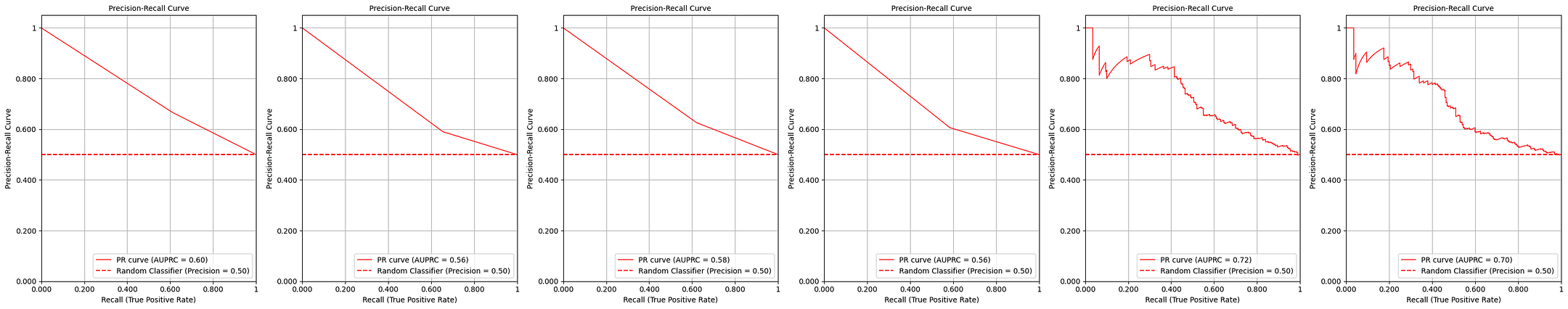
Overall, the Keras Sequential model, optimized with SGD, achieved the best performance with an AUPRC (Area Under Precision-Recall Curve) of 0.72.

Precision-Recall Curves for Six Classifier Models (Comparing Custom, MLP, and Keras Sequential Classifiers with SGD and Adam Optimizers (Source: Kuriko Iwai)

Conclusion

In this exploration, we experimented with custom classifiers, Scikit-learn models, and Keras deep learning architectures.

Our findings underscore that effective machine learning hinges on three critical factors:

robust data preprocessing (tailored to objectives and data distribution),
judicious model selection, and
strategic framework or library choices.

Choosing the right framework

Generally speaking, choose MLPClassifier when:

You’re primarily working with tabular data,
You want to prioritize simplicity, quick iteration, and seamless integration,
You have simple, shallow architectures, and
You have a moderate dataset size (manageable on a CPU).

Choose Keras Sequential when:

You’re dealing with image, text, audio, or other sequential data,
You’re building deep learning models such as CNNs, RNNs, LSTMs,
You need fine-grained control over the model architecture, training process, or custom components,
You need to leverage GPU acceleration,
You’re planning for production deployment, and
You want to experiment with more advanced deep learning techniques.

Limitation of MLPs

While Multilayer Perceptrons (MLPs) proved valuable, their susceptibility to computational complexity and overfitting emerged as key challenges.

Looking ahead, we’ll delve into how Recurrent Neural Networks (RNNs) and Convolutional Neural Networks (CNNs) offer powerful solutions to these inherent MLP limitations.

You can find more info about me on my Portfolio / LinkedIn / Github.