Optimizing the Knapsack Problem Using Stochastic Hill Climbing Algorithm

Introduction In this blog, we will explore how to solve the well-known Knapsack Problem using the Stochastic Hill Climbing algorithm. The Knapsack Problem is a classic optimization problem where the goal is to maximize the value of selected items, subject to weight constraints. Specifically, we'll use the stochastic version of the hill climbing algorithm, which is a local search method that helps in finding the optimal or near-optimal solution for such combinatorial optimization problems. ## The Knapsack Problem In the 0/1 Knapsack Problem, you are given a set of items, each with a weight and a value. The goal is to select a subset of these items such that: The total weight of the selected items does not exceed the maximum weight limit of the knapsack. The total value of the selected items is as large as possible. In our case, the problem consists of 10 items, each with a specified price and weight. The objective is to select the items that maximize the total price without exceeding a weight of 10 kg. Algorithm Selection: Stochastic Hill Climbing We will use the Stochastic Hill Climbing algorithm to solve this optimization problem. This variant of the Hill Climbing algorithm adds randomness to the local search process, which allows it to explore the solution space more effectively by not always choosing the best immediate neighbor. This randomness can help avoid local optima and increase the chances of finding the global optimum. Problem Setup We are given two arrays: prices: Contains the values of the items. weights: Contains the weights of the items. We also have a maximum weight limit (max_kg) and a certain number of iterations (epochs) to run the algorithm. Our goal is to find a solution where the total weight is less than or equal to 10 kg, and the total price is maximized. import numpy as np from local_search import LocalSearch import numpy as np import matplotlib.pyplot as plt local_search = LocalSearch() prices = np.array([60, 50, 70, 30, 80, 90, 100, 40, 110, 120]) weights = np.array([0.5, 1.2, 2, 3, 0.7, 0.9, 1.5, 0.2, 0.6, 2.5]) max_kg = 10 epochs = 1000 problem_dimension = 10 def objective_function(solution): total_price = np.sum(np.multiply(prices, solution)) if total_price == 0: return 10000 return 1 / total_price def extra_condition_fn(solution): return np.sum(np.multiply(solution, weights)) = 0.5) for i in inversible_indices[0]: copied_solution[i] = 1- copied_solution[i] neighborhoods.append(copied_solution) return np.array(neighborhoods) def calculate_initial_solution_fn(dim): return np.zeros(dim) epoch_results = local_search.fit(objective_function, epochs, problem_dimension, extra_condition_fn=extra_condition_fn, calculate_initial_solution_fn = calculate_initial_solution_fn, custom_generate_neighbours_fn=custom_generate_neighbours_fn , algorithm_type="stochastic_hill_climbing") np.set_printoptions(precision=3, suppress=True) plt.plot(range(0,1000), 1 / np.array(epoch_results).ravel()) plt.title(f"Best Price: {1 / local_search.best_solution_value} KG: {np.sum(np.multiply(local_search.best_solution, weights))}") plt.xlabel("Iteration") plt.ylabel("Price") plt.show() Results Best Solution Found -> [1 1 1 0 1 1 1 0 1 1] prices = np.array([60, 50, 70, 30, 80, 90, 100, 40, 110, 120]) weights = np.array([0.5, 1.2, 2, 3, 0.7, 0.9, 1.5, 0.2, 0.6, 2.5]) This means that The best price found is calculated as follows: 160 + 501 + 701 + 300 + 801 + 901 + 1001 + 400 + 1101 + 1201 = 680 The best weight found is calculated as follows: 10.5 + 1.21 + 21 + 30 + 0.71 + 0.91 + 1.51 + 0.20 + 0.61 + 2.51 = 9.9 Key Steps in the Code: Objective Function: The goal is to maximize the total price. We define an objective function that takes a solution (a binary array representing selected items) and returns the inverse of the total price. A high penalty is applied when no items are selected. Extra Condition: We add a constraint to ensure that the total weight of the selected items does not exceed the given weight limit. Neighbor Generation: The custom_generate_neighbours_fn function generates neighboring solutions by randomly flipping the selection of items based on probabilities. This randomness helps the algorithm avoid getting stuck in local optima. Initial Solution: The initial solution is defined as selecting no items (all zeros). Stochastic Hill Climbing: The fit() method of LocalSearch runs the algorithm, iterating through epochs and refining the solution until the best solution is found or the maximum number of iterations is reached.

Apr 12, 2025 - 19:54

Optimizing the Knapsack Problem Using Stochastic Hill Climbing Algorithm

Introduction

In this blog, we will explore how to solve the well-known Knapsack Problem using the Stochastic Hill Climbing algorithm. The Knapsack Problem is a classic optimization problem where the goal is to maximize the value of selected items, subject to weight constraints. Specifically, we'll use the stochastic version of the hill climbing algorithm, which is a local search method that helps in finding the optimal or near-optimal solution for such combinatorial optimization problems.

## The Knapsack Problem
In the 0/1 Knapsack Problem, you are given a set of items, each with a weight and a value. The goal is to select a subset of these items such that:

The total weight of the selected items does not exceed the maximum weight limit of the knapsack.
The total value of the selected items is as large as possible.

In our case, the problem consists of 10 items, each with a specified price and weight. The objective is to select the items that maximize the total price without exceeding a weight of 10 kg.

Algorithm Selection: Stochastic Hill Climbing

We will use the Stochastic Hill Climbing algorithm to solve this optimization problem. This variant of the Hill Climbing algorithm adds randomness to the local search process, which allows it to explore the solution space more effectively by not always choosing the best immediate neighbor. This randomness can help avoid local optima and increase the chances of finding the global optimum.

Problem Setup

We are given two arrays:

prices: Contains the values of the items.
weights: Contains the weights of the items.

We also have a maximum weight limit (max_kg) and a certain number of iterations (epochs) to run the algorithm. Our goal is to find a solution where the total weight is less than or equal to 10 kg, and the total price is maximized.

import numpy as np
from local_search import LocalSearch
import numpy as np
import matplotlib.pyplot as plt

local_search = LocalSearch()


prices = np.array([60, 50, 70, 30, 80, 90, 100, 40, 110, 120])
weights = np.array([0.5, 1.2, 2, 3, 0.7, 0.9, 1.5, 0.2, 0.6, 2.5])
max_kg = 10
epochs = 1000
problem_dimension = 10

def objective_function(solution):
    total_price = np.sum(np.multiply(prices, solution))
    if total_price == 0:
        return 10000
    return 1 / total_price


def extra_condition_fn(solution):
    return np.sum(np.multiply(solution, weights)) <= max_kg


def custom_generate_neighbours_fn(neighborhood_count, dim, best_solution):
    neighborhoods = []

    for _ in range(neighborhood_count):
        probs = np.random.uniform(0, 1, dim)
        copied_solution = np.array(best_solution, copy=True)
        inversible_indices = np.where(probs >= 0.5)
        for i in inversible_indices[0]:
            copied_solution[i] = 1- copied_solution[i]
        neighborhoods.append(copied_solution)


    return np.array(neighborhoods)

def calculate_initial_solution_fn(dim):
    return np.zeros(dim)



epoch_results = local_search.fit(objective_function, epochs, 
                                 problem_dimension,
                                 extra_condition_fn=extra_condition_fn,
                                 calculate_initial_solution_fn = calculate_initial_solution_fn,
                                 custom_generate_neighbours_fn=custom_generate_neighbours_fn ,
                                 algorithm_type="stochastic_hill_climbing")

np.set_printoptions(precision=3, suppress=True)

plt.plot(range(0,1000), 1 / np.array(epoch_results).ravel())
plt.title(f"Best Price: {1 / local_search.best_solution_value} KG: {np.sum(np.multiply(local_search.best_solution, weights))}")
plt.xlabel("Iteration")
plt.ylabel("Price")
plt.show()

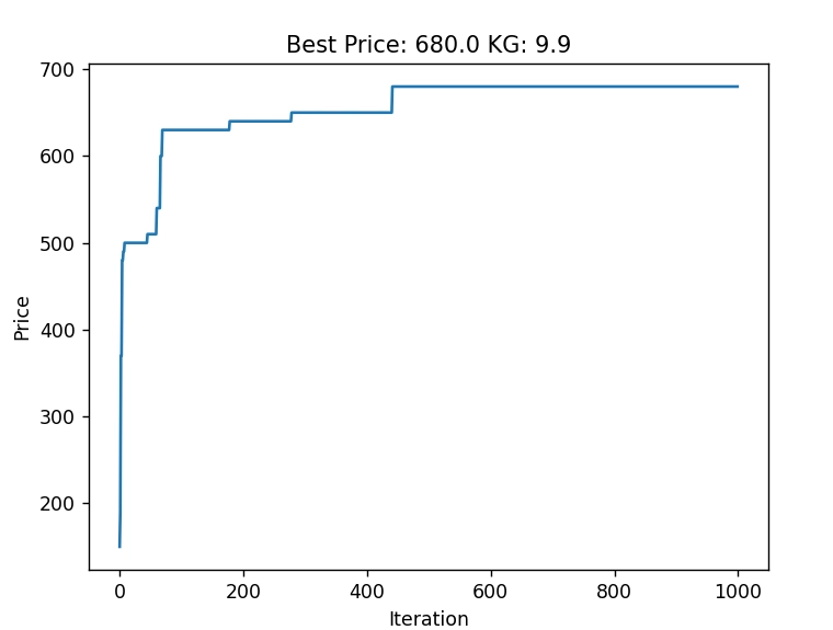
Results

Best Solution Found -> [1 1 1 0 1 1 1 0 1 1]
prices = np.array([60, 50, 70, 30, 80, 90, 100, 40, 110, 120])
weights = np.array([0.5, 1.2, 2, 3, 0.7, 0.9, 1.5, 0.2, 0.6, 2.5])

This means that
The best price found is calculated as follows: 1*60 + 50*1 + 70*1 + 30*0 + 80*1 + 90*1 + 100*1 + 40*0 + 110*1 + 120*1 = 680
The best weight found is calculated as follows: 1*0.5 + 1.2*1 + 2*1 + 3*0 + 0.7*1 + 0.9*1 + 1.5*1 + 0.2*0 + 0.6*1 + 2.5*1 = 9.9

Key Steps in the Code:

Objective Function: The goal is to maximize the total price. We define an objective function that takes a solution (a binary array representing selected items) and returns the inverse of the total price. A high penalty is applied when no items are selected.
Extra Condition: We add a constraint to ensure that the total weight of the selected items does not exceed the given weight limit.
Neighbor Generation: The custom_generate_neighbours_fn function generates neighboring solutions by randomly flipping the selection of items based on probabilities. This randomness helps the algorithm avoid getting stuck in local optima.
Initial Solution: The initial solution is defined as selecting no items (all zeros).
Stochastic Hill Climbing: The fit() method of LocalSearch runs the algorithm, iterating through epochs and refining the solution until the best solution is found or the maximum number of iterations is reached.