Hands-On AI for Beginners: Classifying Iris Flowers in Python

Your First Practical AI Project: Classifying Iris Flowers with Python Embarking on your first machine learning project can feel daunting, but with the right guidance, it's an exciting journey. This article will serve as a hands-on guide, walking you through a classic machine learning task: classifying Iris flowers using Python and the powerful scikit-learn library. By the end, you'll have built, trained, and evaluated a simple classification model, gaining a solid foundation for your future AI endeavors. 1. Understanding the Iris Dataset The Iris dataset is a quintessential "hello world" for machine learning classification. It contains 150 samples of Iris flowers, each belonging to one of three species: Iris setosa, Iris versicolor, and Iris virginica. For each flower, four features are measured: sepal length, sepal width, petal length, and petal width, all in centimeters. Our goal is to build a model that can predict the species of an Iris flower given these four measurements. Let's start by loading this dataset using scikit-learn's built-in utility. from sklearn.datasets import load_iris import pandas as pd import matplotlib.pyplot as plt import seaborn as sns from sklearn.model_selection import train_test_split from sklearn.neighbors import KNeighborsClassifier from sklearn.metrics import accuracy_score, classification_report # 1. Load the Iris dataset iris = load_iris() X = iris.data # Features (sepal length, sepal width, petal length, petal width) y = iris.target # Target (species: 0, 1, or 2) print("Dataset loaded successfully!") print(f"Features shape: {X.shape}") print(f"Target shape: {y.shape}") print("Feature names:", iris.feature_names) print("Target names:", iris.target_names) The output confirms that our dataset has 150 samples and 4 features. The target_names show us the three species our model will learn to distinguish. 2. Data Exploration and Visualization Before building a model, it's always a good practice to explore your data. Visualizations can help us understand the relationships between features and how well the different classes are separated. This step is crucial because it provides insights into the data's structure, which can inform our choice of machine learning algorithms. Let's create a scatter plot to visualize two of the features, for example, 'petal length (cm)' and 'petal width (cm)', colored by species. This will give us a visual intuition of how distinct the different Iris species are based on these measurements. # Convert to DataFrame for easier plotting iris_df = pd.DataFrame(data=X, columns=iris.feature_names) iris_df['species'] = y iris_df['species_name'] = iris.target_names[y] # Create a scatter plot plt.figure(figsize=(8, 6)) sns.scatterplot(x='petal length (cm)', y='petal width (cm)', hue='species_name', data=iris_df, palette='viridis', s=100) plt.title('Iris Petal Length vs. Petal Width by Species') plt.xlabel('Petal Length (cm)') plt.ylabel('Petal Width (cm)') plt.legend(title='Species') plt.grid(True) plt.show() This plot visually demonstrates that Iris setosa flowers are quite distinct from the other two species based on their petal measurements, while Iris versicolor and Iris virginica show some overlap, making their classification slightly more challenging. 3. Data Splitting: Training and Testing Sets A fundamental principle in machine learning is to evaluate your model on data it has never seen before. This is why we split our dataset into two parts: a training set and a testing set. Training Set: Used to train the machine learning model. The model learns patterns and relationships from this data. Testing Set: Used to evaluate the model's performance on unseen data. This gives us an unbiased estimate of how well our model will generalize to new, real-world examples. We use train_test_split from sklearn.model_selection for this purpose. The test_size parameter determines the proportion of the dataset to include in the test split (e.g., 0.2 means 20% for testing, 80% for training). random_state ensures reproducibility of your split. # 3. Split data into training and testing sets X_train, X_test, y_train, y_test = train_test_split(X, y, test_size=0.2, random_state=42) print(f"Training set size: {X_train.shape[0]} samples") print(f"Testing set size: {X_test.shape[0]} samples") 4. Choosing and Training a Classification Model For our first project, we'll use the K-Nearest Neighbors (KNN) algorithm. KNN is a simple, non-parametric, instance-based learning algorithm. At a high level, it classifies a new data point by finding the 'K' nearest data points (neighbors) in the training set and assigning the new point the class that is most common among its neighbors. The 'K' in KNN is a hyperparameter that we choose. We'll initialize KNeighborsClassifier with n_neighbors=3, meaning it will consider the 3 closest neighbors. Then, we fit the model to our training data. # 4. Choo

Jun 14, 2025 - 13:50

Hands-On AI for Beginners: Classifying Iris Flowers in Python

Your First Practical AI Project: Classifying Iris Flowers with Python

Embarking on your first machine learning project can feel daunting, but with the right guidance, it's an exciting journey. This article will serve as a hands-on guide, walking you through a classic machine learning task: classifying Iris flowers using Python and the powerful scikit-learn library. By the end, you'll have built, trained, and evaluated a simple classification model, gaining a solid foundation for your future AI endeavors.

1. Understanding the Iris Dataset

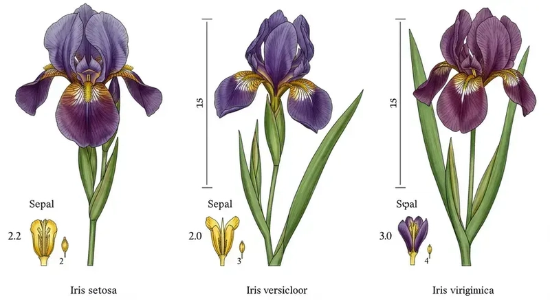
The Iris dataset is a quintessential "hello world" for machine learning classification. It contains 150 samples of Iris flowers, each belonging to one of three species: Iris setosa, Iris versicolor, and Iris virginica. For each flower, four features are measured: sepal length, sepal width, petal length, and petal width, all in centimeters. Our goal is to build a model that can predict the species of an Iris flower given these four measurements.

Let's start by loading this dataset using scikit-learn's built-in utility.

from sklearn.datasets import load_iris
import pandas as pd
import matplotlib.pyplot as plt
import seaborn as sns
from sklearn.model_selection import train_test_split
from sklearn.neighbors import KNeighborsClassifier
from sklearn.metrics import accuracy_score, classification_report

# 1. Load the Iris dataset
iris = load_iris()
X = iris.data  # Features (sepal length, sepal width, petal length, petal width)
y = iris.target # Target (species: 0, 1, or 2)

print("Dataset loaded successfully!")
print(f"Features shape: {X.shape}")
print(f"Target shape: {y.shape}")
print("Feature names:", iris.feature_names)
print("Target names:", iris.target_names)

The output confirms that our dataset has 150 samples and 4 features. The target_names show us the three species our model will learn to distinguish.

2. Data Exploration and Visualization

Before building a model, it's always a good practice to explore your data. Visualizations can help us understand the relationships between features and how well the different classes are separated. This step is crucial because it provides insights into the data's structure, which can inform our choice of machine learning algorithms.

Let's create a scatter plot to visualize two of the features, for example, 'petal length (cm)' and 'petal width (cm)', colored by species. This will give us a visual intuition of how distinct the different Iris species are based on these measurements.

# Convert to DataFrame for easier plotting
iris_df = pd.DataFrame(data=X, columns=iris.feature_names)
iris_df['species'] = y
iris_df['species_name'] = iris.target_names[y]

# Create a scatter plot
plt.figure(figsize=(8, 6))
sns.scatterplot(x='petal length (cm)', y='petal width (cm)', hue='species_name', data=iris_df, palette='viridis', s=100)
plt.title('Iris Petal Length vs. Petal Width by Species')
plt.xlabel('Petal Length (cm)')
plt.ylabel('Petal Width (cm)')
plt.legend(title='Species')
plt.grid(True)
plt.show()

This plot visually demonstrates that Iris setosa flowers are quite distinct from the other two species based on their petal measurements, while Iris versicolor and Iris virginica show some overlap, making their classification slightly more challenging.

3. Data Splitting: Training and Testing Sets

A fundamental principle in machine learning is to evaluate your model on data it has never seen before. This is why we split our dataset into two parts: a training set and a testing set.

Training Set: Used to train the machine learning model. The model learns patterns and relationships from this data.
Testing Set: Used to evaluate the model's performance on unseen data. This gives us an unbiased estimate of how well our model will generalize to new, real-world examples.

We use train_test_split from sklearn.model_selection for this purpose. The test_size parameter determines the proportion of the dataset to include in the test split (e.g., 0.2 means 20% for testing, 80% for training). random_state ensures reproducibility of your split.

# 3. Split data into training and testing sets
X_train, X_test, y_train, y_test = train_test_split(X, y, test_size=0.2, random_state=42)

print(f"Training set size: {X_train.shape[0]} samples")
print(f"Testing set size: {X_test.shape[0]} samples")

4. Choosing and Training a Classification Model

For our first project, we'll use the K-Nearest Neighbors (KNN) algorithm. KNN is a simple, non-parametric, instance-based learning algorithm. At a high level, it classifies a new data point by finding the 'K' nearest data points (neighbors) in the training set and assigning the new point the class that is most common among its neighbors. The 'K' in KNN is a hyperparameter that we choose.

We'll initialize KNeighborsClassifier with n_neighbors=3, meaning it will consider the 3 closest neighbors. Then, we fit the model to our training data.

# 4. Choose and train a model
# We'll use KNeighborsClassifier, a simple and intuitive algorithm.
# n_neighbors specifies the 'K' in K-Nearest Neighbors.
knn = KNeighborsClassifier(n_neighbors=3)

# Train the model using the training data
knn.fit(X_train, y_train)

print("K-Nearest Neighbors model trained successfully!")

You can find more details about KNeighborsClassifier in the scikit-learn documentation: https://scikit-learn.org/stable/modules/generated/sklearn.neighbors.KNeighborsClassifier.html

5. Model Evaluation

After training, we need to evaluate how well our model performs. We do this by making predictions on the X_test data (which the model has not seen during training) and comparing these predictions to the actual y_test labels.

Accuracy Score: This is the simplest metric, representing the proportion of correctly classified samples.
Classification Report: Provides a more detailed breakdown of performance per class, including precision, recall, and F1-score.
- Precision: The ability of the classifier not to label as positive a sample that is negative (i.e., out of all predicted positives, how many were truly positive).
- Recall: The ability of the classifier to find all the positive samples (i.e., out of all actual positives, how many were correctly identified).
- F1-score: The harmonic mean of precision and recall, providing a single metric that balances both.

These metrics are essential for understanding your model's strengths and weaknesses, especially in cases where classes might be imbalanced. You can learn more about these fundamental machine learning concepts on the AI & Machine Learning Basics website.

# 5. Make predictions on the test set
y_pred = knn.predict(X_test)

# Evaluate the model's accuracy
accuracy = accuracy_score(y_test, y_pred)
print(f"Model Accuracy on test set: {accuracy:.2f}")

# Display a detailed classification report
print(\"\nClassification Report:\")
print(classification_report(y_test, y_pred, target_names=iris.target_names))

A high accuracy score (close to 1.00) indicates a good model. The classification report gives us a per-class breakdown, which is very useful.

6. Making Predictions on New Data

Now that our model is trained and evaluated, we can use it to predict the species of new, unseen Iris flowers. Imagine you have measurements for a new flower and want to know its species.

# 7. Make a prediction on new data
# Let's create a hypothetical new Iris flower with its measurements
# Format: [[sepal length, sepal width, petal length, petal width]]
new_flower_measurements = [[5.0, 3.3, 1.5, 0.2]] # These measurements are very similar to an Iris Setosa

# Use the trained KNN model to predict the species
predicted_species_index = knn.predict(new_flower_measurements)

# Get the actual species name from the target_names list
predicted_species_name = iris.target_names[predicted_species_index][0]

print(f"\nMeasurements for new flower: {new_flower_measurements[0]}")
print(f"Predicted species for new flower: {predicted_species_name}")

This demonstrates the practical application of your trained model!

Further Exploration

Congratulations! You've successfully completed your first practical AI project. But the journey doesn't end here. Here are some next steps to deepen your understanding and skills:

Try Different Algorithms: Experiment with other classification algorithms available in scikit-learn, such as DecisionTreeClassifier, SVC (Support Vector Machine), or LogisticRegression. Each algorithm has its strengths and weaknesses, and understanding them is key to becoming a proficient machine learning practitioner.
Hyperparameter Tuning: The n_neighbors value in KNN is a hyperparameter. Try different values (e.g., 1, 5, 10, 15) and observe how the model's accuracy changes. This process, known as hyperparameter tuning, is crucial for optimizing model performance.
Vary test_size: Change the test_size parameter in train_test_split (e.g., 0.1, 0.3) and see how it affects your model's evaluation metrics. A smaller test set might lead to a less reliable evaluation.
Explore Other Datasets: Scikit-learn offers many other toy datasets (e.g., load_digits for handwritten digits, load_breast_cancer for medical diagnosis). You can also find numerous datasets on platforms like Kaggle for more complex challenges.
- GeeksforGeeks Machine Learning Projects
- DataCamp Machine Learning Projects

By continuously experimenting and building, you'll solidify your understanding of machine learning concepts and gain confidence in tackling more complex AI projects. Happy coding!