Generative AI Interview for Senior Data Scientists: 50 Key Questions and Answers

I’ve compiled 50 key questions and answers as a technical interview prep guide for senior data scientists in the field of generative AI. I. Transformer Basics Describe the main components of the Transformer architecture and explain how they overcome the limitations of RNNs/LSTMs. Transformers overcome the parallel processing limitations and difficulty in capturing long-range dependencies of RNNs/LSTMs, which rely on sequential processing, through the self-attention mechanism. Self-attention simultaneously calculates the relationships between all token pairs in a sequence, enabling parallel processing and helping each token understand the context by utilizing information from the entire sequence. The main components are: Self-Attention: Each token assesses its relevance to all other tokens in the sequence, effectively capturing long-range dependencies and generating representations rich in contextual information. Multi-Head Attention (MHA): Performs self-attention multiple times in parallel. Each 'head' focuses on different feature subspaces or relationships in the input data, helping the model learn more diverse and complex patterns. Position-wise Feed-Forward Network (FFN): A fully connected neural network applied independently to the representation of each token after passing through the attention layer. It increases the model's representational power and adds computational depth through non-linear transformations. Add & Norm: Applies Residual Connections (adding the input and output of each sub-layer: self-attention, FFN) and Layer Normalization. This is essential for mitigating the vanishing/exploding gradient problem in deep networks and stabilizing training. Positional Encoding: Injects token position information into the self-attention mechanism, which lacks sequence order awareness, allowing the model to recognize the sequence order. Thanks to the combination of these components, especially the parallelizable design, Transformers can effectively scale to large datasets and model sizes. Explain the self-attention mechanism in detail. How is the attention matrix calculated using Query, Key, and Value vectors? Self-attention is a mechanism that calculates weights indicating how relevant every other token in the input sequence is to the current token being processed. For each input token, three vectors are generated through learnable linear transformations: Query (Q), Key (K), and Value (V). The process for calculating attention weights is as follows: Score Calculation: Compute the similarity between the Query vector (Q) of the current token and the Key vectors (K) of all tokens in the sequence (including itself). Typically, the Scaled Dot-Product Attention method is used, which involves taking the dot product and then dividing by the square root of the Key vector dimension. This yields the Attention Score. Normalization: Apply the Softmax function to the calculated attention scores to create Attention Weights, which form a probability distribution summing to 1. These weights indicate how much 'attention' the current token should pay to each other token. Weighted Sum: Compute a weighted average of the Value vectors (V) of all tokens, using their corresponding attention weights, to generate the final output representation for the current token. Through this process, each token obtains a rich representation that effectively incorporates contextual information from its surroundings. How does Multi-Head Attention differ from single-head attention? What are its advantages? Unlike single-head attention which performs a single attention operation, Multi-Head Attention (MHA) performs the attention mechanism multiple times in parallel. Each 'head' learns independent Query, Key, and Value projection matrices, allowing it to focus on different feature subspaces (e.g., syntactic relationships, semantic similarity) or representational aspects of the input data. The attention outputs calculated from each head are concatenated and then passed through an additional linear transformation to form the final output. The main advantage of MHA is that it allows the model to simultaneously process and integrate information from various perspectives, enabling it to capture richer and more complex relationships than a single head could. This ultimately enhances the model's representational power and performance, and can also contribute to stabilizing the learning process. Why is Positional Encoding necessary? Compare absolute and relative methods (e.g., RoPE, ALiBi). Since the self-attention mechanism in Transformers does not consider the order of tokens (permutation invariance), Positional Encoding must be explicitly injected to allow the model to understand the position information of tokens within the sequence. Absolute Positional Encoding: Assigns a unique encoding vector to each token based on its fixed absolute position in the sequence. Examples include the sine and cosine

May 6, 2025 - 14:26

Generative AI Interview for Senior Data Scientists: 50 Key Questions and Answers

I’ve compiled 50 key questions and answers as a technical interview prep guide for senior data scientists in the field of generative AI.

I. Transformer Basics

Describe the main components of the Transformer architecture and explain how they overcome the limitations of RNNs/LSTMs.

Transformers overcome the parallel processing limitations and difficulty in capturing long-range dependencies of RNNs/LSTMs, which rely on sequential processing, through the self-attention mechanism. Self-attention simultaneously calculates the relationships between all token pairs in a sequence, enabling parallel processing and helping each token understand the context by utilizing information from the entire sequence. The main components are:
- Self-Attention: Each token assesses its relevance to all other tokens in the sequence, effectively capturing long-range dependencies and generating representations rich in contextual information.
- Multi-Head Attention (MHA): Performs self-attention multiple times in parallel. Each 'head' focuses on different feature subspaces or relationships in the input data, helping the model learn more diverse and complex patterns.
- Position-wise Feed-Forward Network (FFN): A fully connected neural network applied independently to the representation of each token after passing through the attention layer. It increases the model's representational power and adds computational depth through non-linear transformations.
- Add & Norm: Applies Residual Connections (adding the input and output of each sub-layer: self-attention, FFN) and Layer Normalization. This is essential for mitigating the vanishing/exploding gradient problem in deep networks and stabilizing training.
- Positional Encoding: Injects token position information into the self-attention mechanism, which lacks sequence order awareness, allowing the model to recognize the sequence order.
Thanks to the combination of these components, especially the parallelizable design, Transformers can effectively scale to large datasets and model sizes.
Explain the self-attention mechanism in detail. How is the attention matrix calculated using Query, Key, and Value vectors?

Self-attention is a mechanism that calculates weights indicating how relevant every other token in the input sequence is to the current token being processed. For each input token, three vectors are generated through learnable linear transformations: Query (Q), Key (K), and Value (V). The process for calculating attention weights is as follows:
1. Score Calculation: Compute the similarity between the Query vector (Q) of the current token and the Key vectors (K) of all tokens in the sequence (including itself). Typically, the Scaled Dot-Product Attention method is used, which involves taking the dot product and then dividing by the square root of the Key vector dimension. This yields the Attention Score.
2. Normalization: Apply the Softmax function to the calculated attention scores to create Attention Weights, which form a probability distribution summing to 1. These weights indicate how much 'attention' the current token should pay to each other token.
3. Weighted Sum: Compute a weighted average of the Value vectors (V) of all tokens, using their corresponding attention weights, to generate the final output representation for the current token. Through this process, each token obtains a rich representation that effectively incorporates contextual information from its surroundings.
How does Multi-Head Attention differ from single-head attention? What are its advantages?

Unlike single-head attention which performs a single attention operation, Multi-Head Attention (MHA) performs the attention mechanism multiple times in parallel. Each 'head' learns independent Query, Key, and Value projection matrices, allowing it to focus on different feature subspaces (e.g., syntactic relationships, semantic similarity) or representational aspects of the input data. The attention outputs calculated from each head are concatenated and then passed through an additional linear transformation to form the final output.
The main advantage of MHA is that it allows the model to simultaneously process and integrate information from various perspectives, enabling it to capture richer and more complex relationships than a single head could. This ultimately enhances the model's representational power and performance, and can also contribute to stabilizing the learning process.
Why is Positional Encoding necessary? Compare absolute and relative methods (e.g., RoPE, ALiBi).

Since the self-attention mechanism in Transformers does not consider the order of tokens (permutation invariance), Positional Encoding must be explicitly injected to allow the model to understand the position information of tokens within the sequence.
- Absolute Positional Encoding: Assigns a unique encoding vector to each token based on its fixed absolute position in the sequence. Examples include the sine and cosine functions proposed in the original Transformer paper, or learning embeddings for each position. While simple to implement, a drawback is potentially poorer generalization to sequence lengths unseen during training.
- Relative Positional Encoding: Encodes the relative distance or relationship between tokens instead of their absolute positions. This is often done directly within the attention mechanism.
  - RoPE (Rotary Position Embedding): Reflects relative position information by applying rotational transformations to the Query (Q) and Key (K) vectors based on the token's position.
  - ALiBi (Attention with Linear Biases): Models relative distance by adding a penalty (bias) proportional to the distance between tokens when calculating attention scores.
Relative methods generally tend to generalize better to varying sequence lengths and are preferred in modern Transformer architectures. ALiBi, in particular, is noted for its ease of implementation.
Distinguish between Encoder-only (e.g., BERT), Decoder-only (e.g., GPT), and Encoder-Decoder (e.g., T5) architectures. Describe their typical application areas.

Transformers are broadly classified into three architectures based on how their components (encoder, decoder) are combined, each with different information processing styles and primary applications.
- Encoder-Only Architecture (e.g., BERT): Processes the entire input sequence at once, considering bidirectional context (both preceding and succeeding tokens) when calculating the representation for each token. Primarily used for Natural Language Understanding (NLU) tasks where a deep understanding of the entire input is crucial (e.g., text classification, named entity recognition, question answering).
- Decoder-Only Architecture (e.g., GPT): Operates in an autoregressive manner, generating the output sequence one token at a time. When predicting each token, it only references the previously generated tokens (unidirectional or causal attention). Excels at Natural Language Generation (NLG) tasks like text generation, chatbots, and summarization.
- Encoder-Decoder Architecture (e.g., original Transformer, T5): The encoder processes the input sequence to compress contextual information, and the decoder references this information (typically via cross-attention) to generate the output sequence. Suitable for sequence-to-sequence tasks that transform an input sequence into a different output sequence (e.g., machine translation, document summarization).
What are the computational limitations of the vanilla Transformer, and what approaches exist to address them?

The main computational limitation of the Vanilla Transformer is that the self-attention operation's computation and memory requirements grow quadratically (O(N²)) with the sequence length (N). This is because attention scores must be calculated and stored for every pair of tokens. This makes the computational cost prohibitive for very long sequences (e.g., tens of thousands of tokens or more).
Various approaches have been proposed to overcome this limitation:
- Sparse Attention: Instead of calculating all token pairs, each token attends only to a limited number of other tokens based on a predefined pattern (e.g., neighboring tokens, tokens at specific intervals, some global tokens). This can reduce the complexity to O(N log N) or even O(N).
- Efficient / Linearized Attention: Uses mathematical techniques like kernel methods or low-rank approximation to approximate the attention result without explicitly computing the full attention matrix. Aims for linear or near-linear complexity.
- Hardware Optimization: Does not change the attention calculation itself but improves the actual computation speed by considering hardware characteristics, such as reorganizing the operation order to minimize GPU memory access (read/write) bottlenecks. FlashAttention is a prime example, significantly speeding up exact attention computation.
- Alternative Architectures: Research into new sequence modeling architectures with different scaling properties, such as State Space Models (SSMs), is also actively underway. These methods contribute to improving the scalability of Transformers, allowing them to process longer sequences efficiently and be applied to larger-scale problems.

II. Advanced LLM Architectures and Concepts

What are Scaling Laws (e.g., Kaplan, Chinchilla), and how do they inform pre-training resource allocation?

Scaling Laws describe the empirical relationship where the performance (typically measured by loss) of Large Language Models (LLMs) improves predictably with the resources invested, namely the compute budget, model size (number of parameters), and amount of training data (number of tokens). This relationship is often observed to follow a power law, making it possible to somewhat predict and plan for performance improvements based on resource allocation.
Notably, the Chinchilla paper had a significant impact by suggesting that to achieve optimal performance for a given compute budget, model size (parameters) and training data volume (tokens) should be scaled up together at roughly similar rates. This implies the importance of balancing the model's learning capacity (parameter count) with the content it learns from (data volume). This research suggested that many previous large models might have been oversized relative to their compute budget and undertrained on data ('under-trained' or 'compute-suboptimal'), implying better performance could have been achieved with the same compute budget by using smaller models trained on more data.
Therefore, scaling laws provide crucial empirical guidance for deciding how to allocate limited computational resources between model size and data volume during the pre-training phase. They emphasize that finding the balance point for optimal performance within a given budget is more important than simply building the largest possible model. However, it's important to note that these laws are estimates based on empirical observations, and the actual optimal ratio or degree of performance improvement can vary depending on factors like model architecture, data quality, and the target task.
What are emergent capabilities of LLMs? Provide examples.

Emergent Capabilities of LLMs refer to new abilities that seem to appear suddenly and unpredictably as the model's scale (parameter count, training data, compute) surpasses a certain threshold. These capabilities are not observed or are very weak in smaller models and are characterized by the fact that the model was not explicitly designed or directly trained to possess them.
Key examples include:
- Multi-step arithmetic operations and complex logical reasoning
- The ability to understand and follow complex instructions without specific fine-tuning
- Grasping subtle linguistic nuances like irony and humor
- Generating coherent code
- Chain-of-Thought reasoning, where the model explains its reasoning process step-by-step to solve a problem The discovery of these emergent capabilities provides a strong motivation for scaling up models, but their unpredictable nature also poses challenges for ensuring model safety, reliability, and controllability.
Explain the MoE architecture. What are its pros and cons compared to dense models?

A Mixture of Experts (MoE) model replaces some of the feed-forward network layers in a standard Transformer architecture with multiple, smaller, independent 'expert' networks. For each input token, a learnable routing network dynamically selects a small number of experts (usually 1-2) deemed most suitable to process that token. The outputs of the selected experts are then combined to form the final result.
Pros:
- Scalability: Allows for a significant increase in the total number of model parameters while limiting the number of parameters activated for processing each input token. This enables larger model capacity for roughly the same inference speed.
- Inference Efficiency: Since only a few experts participate in the computation for a given token, the inference computational cost (FLOPs) is much lower compared to a dense model of similar total parameter count.
- Expert Specialization: Potential for each expert network to learn to specialize in processing specific types of data or patterns.
Cons:
- Training and Implementation Complexity: Requires additional mechanisms (e.g., auxiliary loss functions) for load balancing to ensure all experts are utilized relatively evenly (avoiding situations where some experts are overused while others are idle). Achieving overall training stability can be challenging.
- Memory Requirement: Although only some experts are used for computation during inference, all expert parameters must be loaded into memory, requiring significantly more memory capacity than a dense model.
- Routing Overhead: The routing computation itself, assigning tokens to experts, can add some computational overhead.
- Parameter Efficiency: Sometimes, achieving the same performance level might require a larger total number of parameters compared to a dense model.
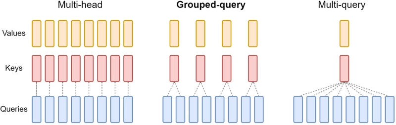
Explain how KV Caching, Multi-Query Attention, and Grouped-Query Attention improve inference efficiency.

KV Caching, Multi-Query Attention, and Grouped-Query Attention are techniques primarily aimed at improving inference efficiency during the autoregressive text generation process of decoder-only models.
- KV Caching: During autoregressive generation, calculating attention for predicting each new token requires attending to all previously generated tokens. KV Caching leverages the fact that the Key and Value vectors for previous tokens do not change. It stores these already computed Key and Value vectors in memory (cache) and reuses them in subsequent steps. This significantly reduces the computation by avoiding repeated Key/Value calculations for the entire sequence at every step. However, a drawback is that the memory occupied by the cache grows very large as the sequence length increases.
- Multi-Query Attention (MQA): In standard Multi-Head Attention (MHA), each attention head has its own Key and Value projection matrices. In MQA, all Query heads share a single Key and Value head (i.e., projection matrices). This reduces the size of the KV cache that needs to be stored by a factor equal to the number of heads, leading to significant savings in memory usage and memory bandwidth requirements.
- Grouped-Query Attention (GQA): GQA is a compromise between standard MHA and MQA. It divides the Query heads into several groups, and the Query heads within each group share one Key and Value head. The KV cache size is larger than MQA but much smaller than standard MHA. This allows for significant memory savings while mitigating the potential quality degradation that can occur with MQA, often achieving a better performance balance than MQA.

III. Advanced Training and Fine-tuning Techniques

How do data cleaning, preprocessing, and tokenizer choice (e.g., BPE) impact LLM training and performance?

Data quality and the way it's processed have a decisive impact on LLM training outcomes and final performance. Since the model learns directly from the provided data, any flaws, biases, or noise within the data will also be learned. Therefore, meticulous data preprocessing is essential for high-quality LLMs. Key steps include:
- Data Cleaning: Correcting noise (e.g., removing HTML tags), inconsistencies, and formatting errors.
- Deduplication: Removing duplicate content within the training data to improve learning efficiency and prevent the model from simply memorizing data.
- Quality Filtering: Identifying and removing low-quality or inappropriate content (e.g., profanity, spam).
- Handling Personal and Sensitive Information: Removing or masking personally identifiable information (PII) or sensitive content.
Tokenizer Choice is also crucial. The tokenizer converts text into integer sequences (token IDs) that the model can understand. Subword-based tokenizers like Byte Pair Encoding (BPE) are widely used. BPE progressively merges frequent pairs of characters to build a vocabulary.
- Vocabulary Size: A larger vocabulary can compress text into fewer tokens, reducing sequence length and potentially improving computational efficiency, but it comes with the trade-off of increasing the model's embedding matrix size and thus memory requirements.
- Efficiency and Performance: Using an efficient tokenizer well-suited to the data characteristics (e.g., code, multilingual text) can reduce sequence lengths, lower computational load, and increase the effective context length the model can handle. Conversely, an inappropriate tokenizer can lead to degraded model performance and sometimes even security vulnerabilities.
What techniques help stabilize the training of large Transformers?

Training very large Transformer models can be unstable, often encountering issues like sudden loss spikes or divergence. To mitigate this training instability and ensure stable learning, the following techniques are often used in combination:
- Learning Rate Scheduling: Employing a warm-up phase where the learning rate is gradually increased at the beginning of training, followed by a decay phase (e.g., cosine decay) where the learning rate is progressively decreased, helps stabilize the optimization process.
- Gradient Clipping: Prevents the gradient explosion phenomenon by scaling down the gradient vector if its norm exceeds a certain threshold.
- Using Stable Optimizers: Optimizers like AdamW, which has an improved handling of weight decay compared to standard Adam with L2 regularization, generally provide more stable training.
- Careful Weight Initialization: Properly setting the initial values of model parameters ensures that activations and gradients are within a stable range at the start of training.
- Layer Normalization: A key component within Transformer blocks that normalizes the distribution of activation values, stabilizing signal propagation throughout the network.
- Using Appropriate Numerical Precision: Using BFloat16 instead of standard 16-bit floating-point (FP16), or employing mixed precision training (using higher precision for critical parts like optimizer states) can enhance numerical stability.
How does instruction tuning differ from general SFT? What is rejection sampling?

Supervised Fine-tuning (SFT) refers to the general process of fine-tuning a pre-trained model using labeled examples (input and correct output pairs) for a specific task.
Instruction Tuning is a form of SFT characterized by training data consisting of explicit 'instructions' and their corresponding 'desired outputs' (e.g., "Summarize the following sentence: [Long sentence]" → "[Summarized sentence]"). The goal of instruction tuning goes beyond improving performance on specific downstream tasks; it aims to teach the model the general ability to understand and follow diverse forms of natural language instructions. This enhances the model's versatility and improves its zero-shot or few-shot generalization performance on unseen new tasks.
Rejection Sampling is one of the data curation techniques used to improve the quality of datasets for instruction tuning or general SFT. The process is as follows:
1. Generate multiple candidate responses for a given instruction (prompt) using the current model.
2. Evaluate the quality of each response using predefined criteria (e.g., a separate reward model score, satisfaction of specific rules, human evaluation).
3. Select only the response(s) with the highest evaluation score, i.e., the best quality response(s), to include in the final fine-tuning dataset. This helps filter out low-quality responses and train the model only on high-quality examples, thereby improving the final model's performance and alignment level.
Compare and contrast alignment methods like RLHF, RLAIF, and DPO/GRPO. What are their core mechanisms, pros, and cons?

Various techniques are used for 'alignment', the process of making LLMs conform to human intentions and values – i.e., making them helpful, honest, and harmless. Here's a comparison of key methods:
- Reinforcement Learning from Human Feedback (RLHF):
  - Core Mechanism: 1) Human evaluators select their preferred response among several generated by the LLM, creating preference data. 2) This data is used to train a separate 'Reward Model (RM)' that predicts which response is better. 3) This RM is used as the reward function in a reinforcement learning (RL, e.g., PPO) algorithm to fine-tune the original LLM.
  - Pros: Can capture nuanced human preferences directly, potentially leading to high alignment quality.
  - Cons: High cost of collecting human preference data, complex overall process, final performance heavily depends on the quality of the learned reward model.
- Reinforcement Learning from AI Feedback (RLAIF):
  - Core Mechanism: Similar to RLHF, but uses a powerful AI model instead of costly human evaluators to generate preference labels. The subsequent process is the same as RLHF (train RM on AI-generated data -> fine-tune LLM with RL).
  - Pros: Easier to scale preference data generation.
  - Cons: Final alignment quality depends on the performance and biases of the AI model used for labeling.
- Direct Preference Optimization (DPO):
  - Core Mechanism: Directly fine-tunes the LLM using preference data (preferred response, dispreferred response pairs), without the need for a separate reward model training or reinforcement learning step. Uses a specific loss function to directly increase the probability of generating preferred responses and decrease the probability of dispreferred ones.
  - Pros: Much simpler to implement and more stable to train than RLHF/RLAIF.
  - Cons: May sometimes struggle to achieve the same level of fine-grained control or peak performance as RLHF.
- Group Relative Policy Optimization (GRPO):
  - Core Mechanism: An RL-based approach that utilizes relative preferences between groups of multiple responses instead of individual responses. Notably, instead of explicitly training a separate value/critic model, it uses statistics of response scores within a group (e.g., the mean) as an implicit baseline for calculating policy gradients.
  - Pros: Can improve resource efficiency (e.g., memory during training) by eliminating the need for a separate value model.
  - Cons: Relatively newer methodology; application and optimization might require specific expertise.
In summary, RLHF and RLAIF combine reward modeling and RL, differing in the feedback source (human/AI). DPO seeks simplicity by skipping reward modeling and RL. GRPO improves resource efficiency within the RL framework through group comparisons and efficient baseline estimation. The suitable method depends on the target alignment level, available data, compute resources, and implementation complexity.
What are the key considerations when designing a reward model for RLHF?.
The success of RLHF heavily relies on the quality of the reward model (RM), which acts as a proxy for human judgment during LLM fine-tuning. Key considerations when designing and training an effective RM include:
- Quality and Diversity of Preference Data: If the human preference data used for training is low-quality or biased in a specific direction, the learned RM will also be biased or inaccurate, negatively impacting the final alignment outcome. Ensuring high-quality, diverse, and consistent data is crucial.
- Reflecting Preference Strength: Ideally, the RM should capture not just the binary judgment of which response is better, but also the strength of that preference (how much better).
- Calibration: It's important to calibrate the RM so that the difference in scores it outputs accurately reflects the difference in preference strength perceived by humans. An uncalibrated RM can misguide the optimization process.
- Model Architecture and Loss Function: Careful selection of the RM's architecture (often initialized based on the target LLM) and the loss function used for training is necessary.
- Preventing Reward Hacking: The RM should be robust against 'reward hacking,' where the LLM exploits loopholes or incorrectly learned patterns in the RM to get high scores, rather than genuinely adhering to human preferences.
- Difficulty of Evaluating the RM: Evaluating the performance of the RM itself is challenging. High prediction accuracy on preference pairs doesn't necessarily guarantee the quality of the final aligned LLM.
- Generalization Performance: The RM must generalize well, accurately predicting human preferences for unseen responses, not just overfitting to the training data.
What is the difference between RLHF and RLVR in training reasoning models, and which approach was primarily used in the development of DeepSeek-R1?.
RLHF and RLVR (Reinforcement Learning from Verifiable Rewards) are both methods for improving LLMs using reinforcement learning, but they differ fundamentally in how rewards are defined and provided.
- RLHF: The reward is based on subjective human preferences. Human evaluators judge the relative quality of model responses (e.g., which is more helpful, safe), and a learned reward model provides the reward signal during RL. Primarily used to improve subjective and complex qualities like conversational ability, style, and safety.
- RLVR: The reward is based on objectively verifiable external rules or tools. For example, verifying the correctness of a math problem solution using an external calculator, or checking code executability and test case passing using a compiler, provides the reward. Often does not require training a separate reward model, making the process simpler and the reward criteria clear and objective. Effective for improving task accuracy and rule-following abilities. The development of DeepSeek-R1, particularly for enhancing its reasoning capabilities, primarily leveraged the RLVR approach. In the initial reinforcement learning phase, reasoning abilities were intensively trained using rule-based 'accuracy rewards' (checking math answers, code execution results) and 'format rewards' (a type of RLVR encouraging the model to generate reasoning steps within specific tags like , ). Subsequently, in the final stages, RLHF (or a similar reward model-based approach) was used supplementarily on top of the established reasoning skills to further improve the model's overall conversational ability, helpfulness, and harmlessness. Therefore, RLVR played a pivotal role in enhancing DeepSeek-R1's reasoning capabilities, with RLHF contributing as a complementary step.
Explain PEFT methods like LoRA/QLoRA. Why are they used, and what problem does QLoRA specifically solve?

Parameter-Efficient Fine-tuning (PEFT) techniques are methodologies for adapting a pre-trained large language model to specific tasks or requirements by updating only a very small subset of the model's parameters, instead of fine-tuning the entire model. This significantly reduces the computational resources, especially memory usage, required for fine-tuning.
- LoRA (Low-Rank Adaptation): One of the most popular PEFT techniques. The core idea is to freeze the original weights of the pre-trained model and add small, trainable 'adapter' matrices to specific layers (typically attention layers). These adapters usually represent the change in the original weight matrix as the product of two low-rank matrices, and only these small adapter matrices are trained during fine-tuning.
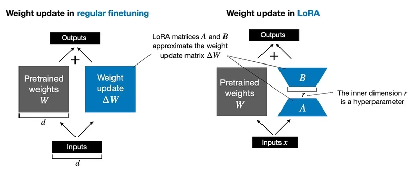
- QLoRA (Quantized LoRA): A technique based on LoRA that further dramatically reduces memory usage. The key is to quantize the weights of the frozen, large base model to a very low precision, such as 4-bit, when loading it into memory. Gradient computation occurs through these quantized weights, but the actual updates are still applied only to the small LoRA adapters, which are kept at a higher precision (e.g., BFloat16). It additionally uses memory optimization techniques like double quantization and paged optimizers. QLoRA enables fine-tuning of very large models (tens to hundreds of billions of parameters) even in memory-constrained environments (e.g., a single consumer GPU), greatly increasing the accessibility of LLMs.
Briefly explain techniques for merging fine-tuned models (e.g., Task Arithmetic, SLERP) and their purpose.

Model Merging typically refers to techniques that combine the parameters of two or more models fine-tuned from the same base model to create a new single model without additional training. The main purposes are:
- Combining Multiple Capabilities: Merging models specialized for different tasks (e.g., coding ability, conversational ability) to create a more versatile model.
- Performance Improvement: Hoping to integrate the strengths of individual models to improve generalization performance.
- Deployment Simplification: Deploying a single merged model instead of multiple specialized ones increases manageability.
Key merging techniques include:
- Weight Averaging: The most basic method, calculating a simple or weighted average of the parameters of each model.
- SLERP (Spherical Linear Interpolation): Instead of simple linear interpolation (a straight line) in the parameter vector space, this technique interpolates along an arc on a sphere, attempting to find a more natural intermediate point.
- Task Arithmetic: Calculates the difference between the fine-tuned model and the original base model parameters, termed the 'task vector'. These vectors are then added to or subtracted from (sometimes with weights) the original model.
- Advanced Merging Techniques: To address issues like parameter interference (e.g., sign conflicts) when merging multiple models, more sophisticated methods have been proposed. Techniques like TIES-Merging or DARE use strategies such as pruning redundant or conflicting parameters, resolving sign conflicts, or selectively resetting parameter values.
These model merging techniques offer ways to effectively combine already learned knowledge and capabilities without the cost of additional training.
What are the core technical challenges and practical trade-offs encountered when designing systems for continuous pre-training or continual learning, and what approaches are commonly used to mitigate these issues?

Continuous Pre-training or Continual Learning aims to incrementally update models with new incoming data over time, instead of periodically retraining them from scratch. Building and operating such systems involves significant technical challenges and trade-offs:
- Catastrophic Forgetting: The phenomenon where a model abruptly loses previously learned knowledge or skills as it learns new data or tasks. This is the most fundamental problem in continual learning. Mitigation strategies include regularization techniques, replay methods (rehearsing some old data), and methods that estimate parameter importance to constrain updates.
- Computational Efficiency: The process of updating a large model with new data must be efficient enough to avoid excessive computational costs. It needs to be significantly cheaper than full retraining to be worthwhile.
- Data Management Complexity: Managing a continuous stream of incoming data is complex. It requires data quality control, storage, deduplication, and handling 'data drift' (changes in data distribution over time).
- Training Stability: Ensuring that the model training remains stable and converges during the continuous update process, without becoming unstable or diverging, can be difficult.
- Evaluation Challenges: Evaluating model performance becomes more complex, as it requires measuring not only the ability to learn new data but also the retention of old knowledge (resistance to forgetting).
- Architectural Suitability: Current standard Transformer architectures may not be inherently optimal for continual learning. Research into dynamic architectures or modular structures that facilitate continuous learning is needed.
- Alignment Maintenance: As the model is continuously updated, it's crucial to continuously monitor and manage its alignment (helpfulness, honesty, harmlessness) to ensure it doesn't degrade or drift in undesirable ways, especially if new data isn't fully curated.
Due to these challenges, continual learning systems often involve trade-offs between performance (acquiring new knowledge), stability (retaining old knowledge), and computational cost.

IV. Retrieval-Augmented Generation

What are the main components of an RAG system? When is RAG preferred over fine-tuning?

Retrieval-Augmented Generation (RAG) is a technique where an LLM, before generating an answer, first retrieves relevant information from an external knowledge source and then uses this retrieved information as context to generate the final response. This helps improve the accuracy of the LLM's answers, incorporate up-to-date information, and reduce hallucinations.
The main components of an RAG system are:
- Retriever: Given a user query (question), its role is to find relevant documents or text passages from a pre-built knowledge base.
- Knowledge Base: The collection of information to be searched. It's built by indexing external documents, database contents, etc.
- Generator: Typically an LLM, which takes the user's original query and the relevant information found by the retriever as combined input, and generates the final answer based on this augmented context.
When RAG is preferred over fine-tuning:
- External Knowledge Integration: Useful when needing to leverage vast, rapidly changing, or domain-specific external knowledge that is difficult to store within the model's parameters.
- Up-to-dateness and Factual Grounding: Can reflect the latest information just by updating the knowledge base (much cheaper than retraining the model), and can cite retrieved documents as evidence, increasing the answer's reliability and providing clear sources.
- Hallucination Reduction: Can reduce hallucinations by guiding the model to base its answers on retrieved facts instead of guessing when it doesn't know something.
- Accessing Specific Information: Effective when needing to accurately reference specific information without the risk of knowledge being forgotten, which can sometimes happen during fine-tuning.
Conversely, fine-tuning is more suitable when the goal is to change the model's inherent characteristics or abilities, such as altering its style, tone, persona, or internalizing specific skills or complex behavioral patterns.
Compare and contrast lexical, semantic, and hybrid search methods.

In RAG systems, the retriever can find relevant information in various ways. The main search methods are:
- Lexical Search:
  - How it works: Primarily based on keyword matching. Uses sparse vector methods (e.g., TF-IDF, BM25) that score documents based on term frequency and distribution within the text.
  - Pros: Computationally efficient, effective at finding documents containing the exact keywords present in the query.
  - Cons: Struggles to grasp semantic similarity (e.g., synonyms, different phrasings). Might treat 'car accident' and 'vehicle collision' as unrelated.
- Semantic Search:
  - How it works: Uses neural network-based language models (encoders, e.g., E5, BGE) to convert queries and documents into dense vectors that capture meaning. Search is performed by finding document vectors closest (most similar) to the query vector in the vector space.
  - Pros: Can find documents that are contextually and semantically similar, even if they don't share exact keywords.
  - Cons: Requires relatively higher computational cost for embedding generation and vector search; performance heavily depends on the quality of the embedding model.
- Hybrid Search:
  - How it works: Combines lexical and semantic search. Strategies include fusing the scores from each method or using one method to retrieve an initial set of candidates and then re-ranking them with the other method.
  - Pros: Can compensate for the weaknesses and leverage the strengths of each method, potentially leading to overall more robust and stable search performance.
  - Cons: Increases system implementation and tuning complexity.
How is RAG performance evaluated (e.g., RAGAS framework)? What are the key metrics?

Evaluating the performance of an RAG system is multifaceted because it requires considering the quality of both the retrieval and generation steps. It involves assessing not just the final answer's quality but also whether each component performs its role well, both individually and holistically. Frameworks like RAGAS attempt to automate and standardize this evaluation process, often leveraging other LLMs as evaluators.
Key evaluation metrics include:
1. Retriever Performance Evaluation:
- Context Precision: Measures the proportion of retrieved documents that are actually relevant to the question. A low score indicates many irrelevant documents were retrieved.
- Context Recall: Measures whether all necessary relevant information required to answer the question was included in the retrieval results. A low score indicates important information was missed.
2. Generator Performance Evaluation:
- Faithfulness: Assesses how well the generated answer aligns with the provided context (retrieved documents), i.e., whether it avoids making things up (hallucinating) that are not supported by the context.
- Answer Relevancy: Evaluates whether the generated answer directly and clearly addresses the user's original question. A low score indicates the answer is verbose or misses the point.
3. End-to-end Evaluation (using ground truth data if available):
- Answer Correctness: Evaluates how well the generated answer matches the actual ground truth or factual answer. (Requires ground truth data)
- Answer Semantic Similarity: Evaluates how semantically similar the generated answer is to the reference (ground truth) answer. (Requires ground truth data)
Using these diverse metrics helps diagnose whether performance bottlenecks in an RAG system stem from the retrieval step, the generation step, or both, guiding improvement efforts.
What are some advanced RAG techniques to improve upon the basic retrieve-then-generate pipeline? How do strategies like query transformation (e.g., HyDE), re-ranking, or iterative retrieval work, and what advantages do they offer over standard RAG?

While basic retrieve-then-generate RAG is effective, it can sometimes suffer from poorly relevant retrieved information or limited ability to answer complex questions. Advanced RAG techniques are used to overcome these limitations and improve performance:
- Query Transformation: Techniques that modify the user's original query to improve retrieval performance, based on the idea that the original query might be suboptimal for searching.
  - HyDE (Hypothetical Document Embeddings): Instead of using the original query, it first uses an LLM to generate a 'hypothetical ideal document' that would answer the query. This generated document, being content-rich, is then embedded and used for searching, increasing the likelihood of finding relevant actual documents compared to using the original query alone. Particularly effective for short or ambiguous queries.
  - Other methods include decomposing the query into sub-queries or extracting/expanding key terms within the query.
- Re-ranking: Often, the initial retrieval step uses a relatively simple method to retrieve a larger set of candidate documents quickly. Re-ranking involves applying a more accurate but computationally expensive model (e.g., a cross-encoder that takes query and document together as input) to this initial candidate set to re-calculate relevance scores and adjust the ranking. This improves the average relevance of the documents ultimately passed to the generator (LLM), enhancing answer quality.
- Iterative/Recursive Retrieval: A strategy to handle complex questions where a single retrieval step may not yield sufficient information.
  - How it works: Analyzes the initial retrieval results. If information is deemed insufficient, it generates new queries based on the previous results to perform additional searches. This 'retrieve → analyze → (if needed) generate new query → retrieve' cycle is repeated until enough information is gathered.
  - Advantages: Enables deeper and more comprehensive answers for questions requiring multi-step reasoning or synthesis of information from various perspectives.
Other advanced RAG techniques include Graph RAG (leveraging knowledge graphs), Small-to-Big retrieval (starting with small text chunks and progressively expanding the search scope), etc. These techniques complement the standard RAG pipeline, addressing its weaknesses and maximizing performance for specific types of questions or data.

V. Multimodal Models

How do multimodal models (e.g., CLIP, Flamingo, LLaVA) typically fuse text and image information?

Multimodal models use various information fusion strategies to process and understand information from different modalities like text, images, and audio together. Key approaches include:
- Shared Embedding Space:
  - Example: CLIP
  - How it works: Uses separate encoders to process each modality (e.g., text, image), generating respective embeddings. These embeddings are then trained to be projected into a single shared latent space. Using a contrastive learning objective, embeddings from related data pairs (e.g., an image and its corresponding text caption) are pushed closer together in this shared space, while unrelated pairs are pushed apart. Fusion happens implicitly through proximity in this embedding space.
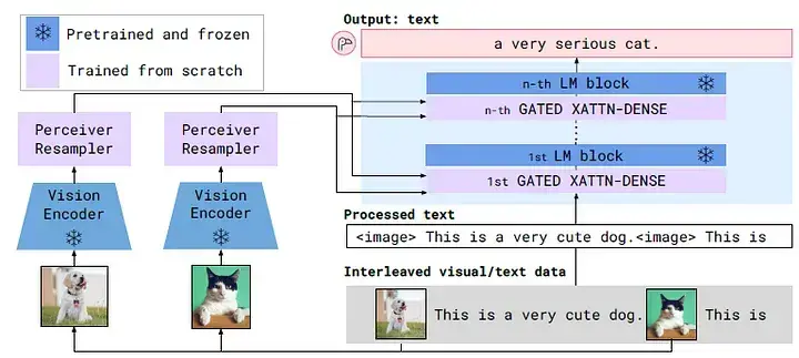
- Cross-Attention:
  - Example: Flamingo
  - How it works: Uses an explicit attention mechanism for information from one modality to directly reference information from another. For instance, cross-attention layers are inserted between specific layers of a pre-trained LLM, allowing text tokens (acting as queries) to directly attend to visual feature tokens (acting as keys/values) extracted by a vision encoder. This enables the active use of visual information during text generation.
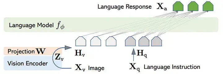
- Input-Level Fusion:
  - Example: LLaVA
  - How it works: Uses a projection layer to transform visual features, extracted via an image encoder (e.g., ViT), into the same dimension as text token embeddings. These transformed visual feature vectors are treated as 'pseudo visual tokens' and are simply concatenated with the text token embedding sequence. A standard LLM (generator) then takes this combined sequence (text tokens + visual tokens) as input, naturally processing and fusing text and visual information together through its internal self-attention mechanisms.
Other approaches involve designing dedicated fusion modules, possibly using gating mechanisms, to merge features at various points in the network.
What are the main challenges in designing/training multimodal models?

Designing and training effective multimodal models presents several key challenges:
- Acquiring High-Quality Large-Scale Datasets: Building large-scale, high-quality datasets where different modalities are well-aligned (e.g., images with accurate, detailed text descriptions) is costly, time-consuming, and difficult. Poor data quality or alignment critically impacts model performance.
- Developing Meaningful Fusion Strategies: Designing effective fusion mechanisms that enable deep integration and cross-modal reasoning, beyond superficial correlations, remains a significant research area.
- High Computational Cost: Multimodal models often include multiple large encoders for each modality (e.g., vision encoder + language model), requiring substantial computational resources for pre-training and fine-tuning.
- Modality Gap: Even when using a shared embedding space theoretically, embeddings from different modalities may tend to form separate clusters within the space in practice. This can hinder seamless information integration between modalities.
- Scalability Issues: Extending the model's capabilities, such as supporting more types of modalities or increasing image/video resolution, can exponentially increase computational and memory requirements, posing significant technical hurdles.
- Evaluation Complexity: Truly evaluating whether a model understands and reasons across modalities, beyond just achieving high scores on specific benchmarks, is difficult. Additionally, interpreting the model's decision-making process and managing potential biases that can be amplified through multi-modal interactions are important challenges.

VI. Image Generation and Diffusion Models

Explain the core principles of the diffusion process. How do Latent Diffusion Models improve efficiency?

Diffusion Models are a powerful family of generative models for creating high-quality images, operating in two stages: the forward process and the reverse process.
1. Forward Process: Gradually adds Gaussian noise to the original data (e.g., a real image) over multiple time steps. After sufficient steps, the data becomes pure noise, indistinguishable from its original form. This process follows a predefined schedule.
2. Reverse Process: Learns a denoising model (typically using a U-Net architecture) to reverse the forward process. This model takes the current noisy data and the corresponding time step as input and predicts the noise that was likely added at that step. During inference (image generation), starting from random noise, the learned denoising model is used to iteratively remove the predicted noise at each step. This progressively denoises the data, eventually generating a clean sample (e.g., a realistic image) similar to the original data distribution.
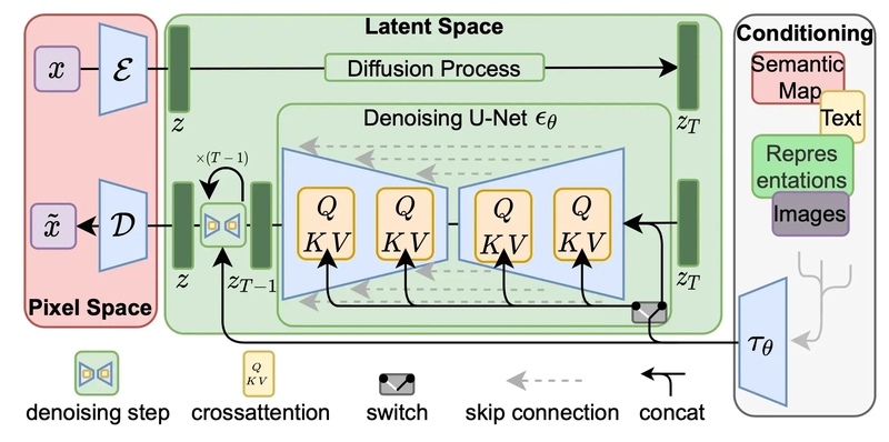
Latent Diffusion Models (LDMs) (the basis for technologies like Stable Diffusion) significantly improve the efficiency of this process. Instead of performing diffusion directly in the high-resolution pixel space, they follow these steps:
- Compression: Uses a pre-trained autoencoder (specifically a VAE) to compress the original high-resolution image into a much lower-dimensional latent space representation.
- Latent Space Diffusion: Performs the forward (noise addition) and reverse (denoising learning and inference) diffusion process entirely within this low-dimensional latent space.
- Reconstruction: After obtaining the final denoised latent vector from the reverse process in the latent space, uses the autoencoder's decoder to reconstruct it back into the original high-resolution pixel space image.
By operating in the low-dimensional latent space instead of the high-dimensional pixel space, LDMs drastically reduce the computational load and memory requirements of the denoising network (U-Net), making high-resolution image generation much faster and more efficient.
What are Diffusion Transformers? How do they differ from traditional U-Net based diffusion models, and what are their potential pros and cons?

Diffusion Transformers (DiTs) refer to models that use a Transformer architecture instead of the traditional U-Net architecture for the reverse denoising process in diffusion models.
Differences from traditional U-Net based models:
- Core Network: U-Nets are based on Convolutional Neural Networks (CNNs) featuring skip connections between downsampling and upsampling paths. In contrast, DiT uses a Transformer, similar to Vision Transformers (ViTs), which divides the image into patches and processes them as a sequence, as the denoising network.
- Input Processing: DiT typically takes the (noised) latent space image patch sequence, time step embeddings, and conditioning information like text embeddings as input. It uses the Transformer's self-attention to learn relationships among these inputs and ultimately predict the noise present in each patch.
Potential Pros:
- Scalability: Transformers have demonstrated excellent scaling properties (performance improvement with increased model size and data) in various domains like NLP and vision. DiT offers the potential to apply the superior scalability of Transformers to diffusion models.
- Leveraging Existing Ecosystem: Can benefit from existing research, pre-training techniques, and optimized implementations related to Transformers.
Potential Cons:
- Loss of Inductive Bias: CNNs inherently possess useful inductive biases for image processing, such as spatial hierarchies. Transformers have relatively fewer such biases (though processing images as patches mitigates this somewhat).
- Computational Cost: The self-attention operation in Transformers can have computation costs that scale with sequence length (though operating in latent space, like in LDMs, significantly reduces this burden).
The relative performance and efficiency of DiT compared to highly optimized U-Net architectures is an active area of research.
What is Classifier-Free Guidance?

Classifier-Free Guidance (CFG) is a technique used in conditional diffusion models, such as text-to-image generation, to steer the generated image to better match the given condition (e.g., text prompt). As the name suggests, it achieves this without requiring a separate classifier model.
How it Works:
1. Training: The diffusion model (noise predictor network) is trained in two ways:
  - Conditional Training: Learns to predict noise given both the noised image and the conditioning information (e.g., text embedding).
  - Unconditional Training: Sometimes (with a certain probability), the conditioning information is removed or replaced with a null value, and the model learns to predict noise based only on the noised image. Thus, the same model learns to predict noise both with and without conditioning.
2. Inference (Image Generation): At each denoising step during image generation, the model calculates two noise predictions: one prediction given the condition, and another prediction without the condition (unconditional).
3. Applying Guidance: The final noise prediction used is a combination of these two. The unconditional prediction is modified by adding the difference between the conditional and unconditional predictions, scaled by a certain weight (the guidance scale, 'w'). A larger 'w' pushes the prediction further in the direction of the conditional prediction (extrapolation).
4. Image Update: The calculated final noise prediction is used to remove noise from the current noisy image to obtain the image for the next step.
Effect: By adjusting the guidance scale 'w', users can control how strongly the generated image adheres to the given condition (text prompt). Higher 'w' values lead to better prompt adherence but might reduce image diversity or quality slightly, while lower 'w' values increase diversity but might decrease relevance to the prompt. CFG is a highly effective technique that allows users to easily control this trade-off between fidelity (to the condition) and diversity.
❓ Origin of the Name: Before CFG, a common method (classifier guidance) involved training a separate classifier model to predict the desired class or attribute from the noisy image. The gradient of this classifier was then used to guide the diffusion process. CFG provides guidance without such a separate classifier, hence the name "Classifier-Free".
Compare and contrast sampling strategies (e.g., DDIM, DPM-Solver) in terms of speed vs. quality.

Diffusion model sampling strategies, or solvers, are algorithms used to generate (sample) images from a trained diffusion model. The original formulation, the DDPM sampler, can produce high-quality images but is very slow, requiring hundreds to thousands of denoising steps. Sampling strategies aim to increase inference speed by using fewer denoising steps while maintaining the highest possible image quality. Here's a comparison of key strategies regarding speed and quality:
- DDIM (Denoising Diffusion Implicit Models):
  - One of the early improved samplers. Allows sampling with much larger time step skips than DDPM, significantly reducing the total number of required steps to the order of tens to hundreds (e.g., 50-250 steps), thus improving speed.
  - Maintains good quality at reasonable step counts but tends to show noticeable quality degradation at very few steps (e.g., below 10-20 steps).
- DPM-Solver (Diffusion Probabilistic Model Solver) family:
  - Interprets the diffusion process as solving a stochastic differential equation (SDE) or ordinary differential equation (ODE) and applies higher-order numerical methods to solve these equations faster and more accurately.
  - Can generate very high-quality images with far fewer steps than DDIM, often just 10-25 steps, offering significant speed improvements for comparable quality.
  - Various variants exist, such as DPM-Solver++ and UniPC, known for good stability, especially when used with CFG.
Conclusion: Currently, DPM-Solver family samplers are generally considered to offer the best trade-off between generation speed and sample quality, greatly enhancing the practicality of diffusion models. The choice of sampler depends on the required quality level and the acceptable generation time.
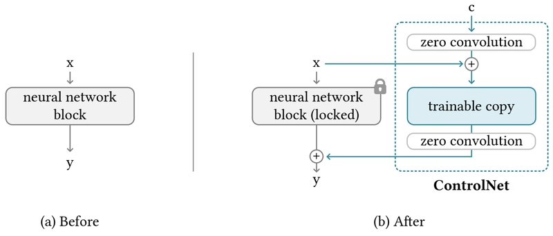
What is ControlNet, and how does it enable controllable image generation?

ControlNet is an add-on neural network module designed to add extra spatial control capabilities to pre-trained large-scale text-to-image diffusion models (like Stable Diffusion). It allows users to provide not only a text prompt but also various types of conditioning images to finely control the structure, shape, pose, etc., of the generated image. Examples of control conditions include:
- Canny edges map
- Depth map
- Human pose skeleton (e.g., OpenPose)
- Semantic segmentation map
- Scribbles, etc.
How it Works & Features:
1. Freezes Base Model: ControlNet does not modify the weights of the existing powerful pre-trained diffusion model at all; they remain frozen.
2. Copies and Trains Encoder Blocks: It duplicates only the encoding part (downsampling blocks) of the base model's denoising network (usually a U-Net) and makes this copy trainable.
3. Inputs Control Condition: The user-provided control condition image (e.g., edge map) is fed into this trainable encoder copy.
4. 'Zero Convolution' Connection: The output features from each block of the trainable copy pass through 'zero convolutions' (1x1 convolution layers initialized with zero weights) and are then added to the input of the corresponding decoding part (upsampling blocks) of the original frozen U-Net.
5. Training: When training ControlNet, only the weights of the copied encoder blocks and the zero convolution layers are updated. Training data consists of (original image, text prompt, control condition image) triplets.
This architecture allows ControlNet to leverage the vast knowledge and generative power of the base model while effectively controlling the spatial structure of the image according to the added condition. The zero convolutions initially allow the base model to operate unaffected, gradually injecting the control information as they are trained.
What are the common fine-tuning techniques used to adapt pre-trained image generation models to specific styles or subjects, and what are the characteristics of each method? Also, what are the key technical challenges to be aware of when applying these techniques?

Several techniques are used to adapt powerful pre-trained image generation models to specific styles, persons, objects, or concepts. Each technique differs in the depth of customization, required data amount, and computational resource needs.
Key Fine-tuning Techniques:
- Full Fine-tuning:
  - Method: Retrains all or most of the model's weights on a new target dataset (e.g., images of a specific style).
  - Characteristics: Allows for fundamental changes to the model's behavior, enabling deep customization. However, it requires substantial computational resources (GPU memory, time) and carries a high risk of catastrophic forgetting, where the model loses its vast pre-trained knowledge or diverse generation capabilities.
- PEFT (Parameter-Efficient Fine-tuning): Freezes most weights and trains only a small subset of parameters, improving resource efficiency. Common techniques in image generation include:
  - LoRA: Adds small, low-rank 'adapter' matrices to specific layers (often attention-related) of the base model and trains only these adapters. Effective for applying specific styles or making fine adjustments with relatively few resources.
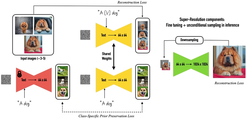
  - DreamBooth: Uses a small number of images (typically 3-5) of a specific subject (e.g., a particular person, pet) and a unique identifier string (e.g., "a photo of sks dog") to teach the model to generate that subject with high fidelity. Updates a subset of the model's weights.
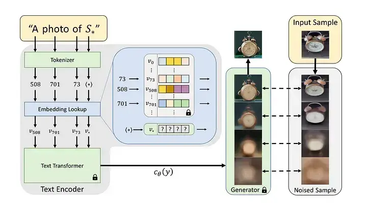
  - Textual Inversion: Does not change the model's weights at all. Instead, it learns a new embedding vector for a new pseudo-word that represents the target concept (style, object). Training is very lightweight and fast, but it might be harder to capture specific subjects as strongly as DreamBooth.
Key Technical Challenges:
Regardless of the fine-tuning technique used, one might face the following challenges:
- Catastrophic Forgetting: The model losing previously learned diverse knowledge and generation capabilities while learning the new style or concept. Particularly prominent in full fine-tuning.
- Overfitting: The model becoming too specialized to the fine-tuning data, resulting in outputs that are overly similar to the training examples or poor generalization to new prompts. Outputs can become repetitive or lack diversity.
- Finding Balance: Striking the delicate balance between achieving the desired level of customization while preserving the model's general generative capabilities and stability is crucial. Careful tuning of learning rates, training data amount, and training steps is required.

VII. Foundation Model Engineering and Infrastructure

Explain data, tensor, and pipeline parallelism. When is each used? What are frameworks like DeepSpeed/FSDP?

Very large models often don't fit into the memory of a single accelerator (like a GPU) or take too long to train on a single device. Therefore, distributed training strategies using multiple devices are essential. Key parallelism techniques include:
- Data Parallelism (DP):
  - Method: Replicates the entire model across multiple devices. Each device processes a different portion (minibatch) of the overall data batch to compute gradients. The gradients are then averaged across all devices (e.g., via an AllReduce operation) to update the model weights simultaneously.
  - When Used: Primarily when the model itself fits on a single device, but you want to speed up training by processing more data in parallel. It's the most basic form of parallelism.
- Tensor Parallelism (TP):
  - Method: Splits individual operations (tensor computations) within the model, such as large matrix multiplications (inside attention or FFN layers), across multiple devices. The weights of a specific layer might be distributed across devices, requiring inter-device communication (e.g., AllReduce, AllGather) during the forward and backward passes for that layer.
  - When Used: When even a single layer of the model is too large to fit into the memory of one device.
- Pipeline Parallelism (PP):
  - Method: Divides the model's layers into multiple sequential stages and assigns each stage to a different device. Data flows through the pipeline from one stage to the next, like an assembly line (passing activations forward, passing gradients backward).
  - When Used: When the entire model (even with tensor parallelism) doesn't fit on a single device, or when you want to reduce the memory burden of storing intermediate computations (activations).
In practice, training very large models often uses a hybrid approach combining these three parallelism techniques. Frameworks like DeepSpeed or PyTorch's FSDP (Fully Sharded Data Parallel) provide tools and abstractions to make implementing and managing these complex parallelism strategies easier, often incorporating memory optimization techniques like ZeRO.
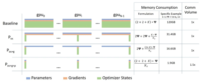
Explain ZeRO stages 1, 2, and 3. How do they reduce memory requirements?

ZeRO (Zero Redundancy Optimizer) is a family of optimization techniques designed to drastically reduce the per-device memory consumption in data parallel (DP) training environments. It achieves this by partitioning the model state information (optimizer states, gradients, model parameters), which would otherwise be redundantly stored on each device (GPU), across multiple devices. This enables training much larger models on limited hardware. ZeRO has three stages of increasing optimization:
- ZeRO Stage 1:
  - Partitions: Optimizer states (e.g., momentum and variance values for AdamW optimizer).
  - How it works: Each device stores only the portion (partition) of the optimizer states corresponding to the subset of model parameters it is responsible for. Standard DP replicates the entire optimizer state on all devices; ZeRO Stage 1 eliminates this redundancy. When parameters need updating, the required optimizer states are fetched via communication.
- ZeRO Stage 2:
  - Partitions: Optimizer states + Gradients.
  - How it works: In addition to partitioning optimizer states (Stage 1), it also partitions the gradients across devices. After the backward pass, each device computes and stores only the gradients for its assigned parameter partition (using a ReduceScatter operation). This saves additional memory compared to standard DP where all devices compute and AllReduce the full gradient tensor.
- ZeRO Stage 3:
  - Partitions: Optimizer states + Gradients + Model parameters.
  - How it works: The highest level of optimization, partitioning the model parameters themselves. Each device holds only its assigned parameter partition in memory for most of the time. When the forward or backward computation for a specific layer is needed, the required parameters are temporarily gathered from all relevant devices via communication (AllGather), used for computation, and then immediately released to free up memory.
  - Effect: Provides the largest memory savings, theoretically enabling training of models almost arbitrarily large, given enough devices.
Higher ZeRO stages offer greater memory savings but typically come with the trade-off of increased inter-device communication as partitioned data needs to be gathered more frequently.
Discuss quantization techniques (PTQ vs QAT) and formats (FP16, BF16, INT8). What are their impacts on performance/size/accuracy? Explain GPTQ/AWQ.

Quantization is the technique of reducing the numerical precision (number of bits) used to represent a model's weights and/or activations. Instead of the standard 32-bit floating-point (FP32), formats like 16-bit floating-point (FP16, BF16) or 8-bit integers (INT8) are used.
Purpose and Effects:
- Reduced Model Size: Uses fewer bits, making model files smaller, which is beneficial for storage and loading.
- Reduced Memory Usage: Less memory is required to load the model during inference. Particularly effective when applied to memory-intensive components like the KV cache.
- Improved Inference Speed: Reduced memory bandwidth usage and potential acceleration from hardware supporting low-precision computations (e.g., Tensor Cores on NVIDIA GPUs) can lead to faster computations.
Key Formats:
- FP16: Uses half the bits of FP32, offering a relatively good balance between speed and accuracy. However, its narrower representable range can lead to overflow/underflow issues.
- BF16 (BFloat16): Also 16-bit, but allocates more bits to the exponent, giving it a wide representable range similar to FP32. Tends to be more numerically stable than FP16 for training and inference.
- INT8: Uses 8-bit integers, offering the potential for the most significant speed improvements and memory savings. However, converting floating-point numbers to integers involves greater information loss, making a careful conversion process (calibration) crucial to minimize accuracy degradation.
Key Quantization Techniques:
- Post-Training Quantization (PTQ): Takes an already trained model and converts its weights (and sometimes activations) to lower precision without retraining. Often uses a small amount of calibration data to find optimal conversion scaling factors. Relatively simple to implement, but can lead to model accuracy loss, especially when quantizing to very low bit-widths (e.g., 4-bit or lower).
  - GPTQ, AWQ: Advanced PTQ techniques specifically developed to effectively quantize LLM weights down to 4-bit precision. They aim to minimize accuracy degradation even at very low bit-widths by considering weight importance and minimizing quantization error.
- Quantization-Aware Training (QAT): Simulates the quantization operations (inserts fake quantization ops) during the model training or fine-tuning process. The model learns to become robust to the errors introduced by quantization, generally achieving higher accuracy than PTQ for the same bit width. However, it requires an additional training process, costing more time and computation.
All quantization techniques involve a trade-off between efficiency gains (speed, memory) and the potential for model performance (accuracy) degradation.
How does speculative decoding speed up LLM inference?

Speculative Decoding is a technique to speed up the inference process of autoregressive LLM text generation (generating one token sequentially after another). The core idea is to use two models together: a small, fast 'draft' model and a large, accurate but slow 'target' model.
How it Works:
1. Draft Generation: Given the sequence generated so far, the small, fast draft model first quickly predicts and proposes a short sequence of candidate tokens (e.g., 3-5 tokens) for the future.
2. Parallel Verification: The large, slow target model takes the entire candidate token sequence proposed by the draft model as input and processes it in parallel in a single forward pass. During this pass, the target model verifies the draft model's proposals by comparing them against what it would have predicted at each position.
3. Token Acceptance: If the target model agrees with the draft model's proposals for the first 'k' consecutive tokens, these 'k' tokens are accepted and appended to the final output sequence all at once.
4. Mismatch Handling: If the target model's prediction differs from the draft model's proposal at the 'k+1'-th token, only the first 'k' agreed-upon tokens are accepted. The 'k+1'-th token is then taken from the target model's prediction. The process then repeats, with the draft model generating the next candidate sequence.
Effect: If the draft model is reasonably accurate, this method allows confirming multiple tokens simultaneously with just one expensive forward pass of the target model. This can result in significant speedups (often 2x-4x or more) compared to the standard autoregressive decoding method where the target model generates only one token per forward pass.
How does FlashAttention improve attention efficiency?
FlashAttention is an algorithm optimized to perform the standard self-attention computation much faster and using less memory, especially for long sequences. It achieves this by efficiently leveraging the characteristics of the GPU memory hierarchy.
Core Principle:
A major performance bottleneck in standard attention implementations often arises not from the raw computation itself, but from writing and reading very large intermediate results (specifically, the N x N attention score matrix, where N is sequence length) to and from the relatively slow main GPU memory (High Bandwidth Memory, HBM).
FlashAttention focuses on minimizing these slow HBM accesses:
1. Tiling: It partitions the input matrices (Query Q, Key K, Value V) into smaller blocks (tiles) that fit into the much faster on-chip GPU memory (SRAM).
2. Computation within SRAM: The attention computation for each block (matrix multiplication of Q and K for scores, softmax application, weighted sum with V) is performed entirely within the fast SRAM. This avoids writing the huge intermediate attention score matrix to the slow HBM. (It uses numerically stable techniques for block-wise softmax calculation).
3. Optimized Backward Pass: For the backward pass during training (gradient calculation), standard attention typically requires storing the large attention matrix computed in the forward pass, consuming significant memory. FlashAttention avoids this by recomputing the necessary parts on-the-fly within SRAM during the backward pass, saving substantial memory at the cost of some extra computation.
In conclusion, FlashAttention employs an IO-aware approach optimized for the GPU memory hierarchy, minimizing HBM reads/writes. This allows it to achieve significant speedups and reduced memory usage while maintaining the exact attention computation results.
What is the purpose of using ONNX or TensorRT for deployment?

When deploying a trained deep learning model into a real-world service environment for inference, optimization to increase execution speed and reduce resource consumption is crucial. ONNX and TensorRT are prominent tools and frameworks widely used for this purpose.
- ONNX (Open Neural Network Exchange):
  - Purpose: An open standard model format designed to provide interoperability between various deep learning frameworks (PyTorch, TensorFlow, etc.).
  - How it works: A model trained in one framework can be converted to the ONNX format. This format can then be run on various hardware or inference engines that support it (e.g., ONNX Runtime). It facilitates easy model transfer and execution even if the development framework and deployment environment differ.
  - Optimization: ONNX Runtime itself performs optimizations like model graph fusion (operator fusion) and leveraging hardware acceleration features to improve inference performance.
- TensorRT:
  - Purpose: A software development kit (SDK) and runtime library provided by NVIDIA specifically designed to maximize inference performance on NVIDIA GPUs.
  - How it works: Takes models developed in various frameworks (often including models converted via ONNX) and performs highly aggressive optimizations specifically tailored for NVIDIA GPU architectures.
  - Key Optimization Techniques:
    - Layer & Tensor Fusion: Combines multiple operations into a single GPU kernel to reduce overhead.
    - Kernel Auto-Tuning: Automatically selects the kernel implementation that yields the fastest performance on the target GPU hardware.
    - Precision Calibration: Optimizes the model to use lower precision formats like FP16 or INT8 for faster execution.
    - Multi-stream execution, dynamic tensor memory management, etc.
  - Result: Generally aims to achieve the lowest latency and highest throughput possible on NVIDIA GPUs.
In summary, ONNX serves as a standard for model interoperability across diverse environments, while TensorRT is a deep optimization tool focused on extracting maximum performance specifically from NVIDIA GPUs. A common workflow involves converting a model to ONNX first, and then further optimizing it with TensorRT.
How do static batching and continuous batching techniques differ for LLM inference, and why does continuous batching often yield better performance in LLM scenarios? Furthermore, explain how technologies like vLLM specifically contribute to the efficient implementation of continuous batching.

During LLM inference, Batching is a crucial technique to improve the efficiency of parallel processing hardware like GPUs by processing multiple user requests together. The two main approaches are static batching and continuous batching.
- Static Batching:
  - Method: Groups incoming requests into batches of a predetermined fixed size. The GPU waits until the computation for the entire batch is completed before processing the next batch.
  - Drawback: LLM response lengths are highly variable per request. In static batching, even short requests that finish early must wait until the longest request in the batch completes its generation. This leads to wasted GPU resources (increased idle time) and increases the average response time for users, making it inefficient.
- Continuous Batching (or Dynamic Batching):
  - Method: Does not use fixed batches but manages requests dynamically. As soon as any request within the group currently being processed by the GPU finishes generating its response, the resources it was using are immediately freed up, and a new waiting request is immediately inserted to utilize those resources for the next computation step.
  - Advantage: Allows the GPU to operate continuously without waiting for the entire group to finish. It effectively addresses the variable output length problem of LLMs, maximizing GPU utilization, reducing average latency, and significantly increasing overall system throughput. This makes it much better suited for real-world service environments with a mix of requests of varying lengths.
Contribution of vLLM and PagedAttention:
While conceptually efficient, implementing continuous batching effectively faced technical challenges, particularly with managing the memory for the KV cache used in Transformer attention. The dynamic addition/removal of requests with varying lengths led to severe memory fragmentation, making it difficult to reuse memory efficiently.
The vLLM library addresses this problem by introducing an innovative technique called PagedAttention.
- PagedAttention: Inspired by operating system memory paging, it manages the KV cache in small, fixed-size blocks (pages) that do not need to be contiguous in physical memory.
- Effect: Each request is allocated only the pages it needs. When a request completes, its pages are immediately returned and can be reused by other requests. This virtually eliminates memory fragmentation, boosting KV cache memory utilization to over 90% and enabling highly efficient implementation of continuous batching.
Consequently, vLLM and PagedAttention play a key role in realizing the theoretical benefits of continuous batching, significantly enhancing LLM inference serving performance.

VIII. Reasoning, Prompting, and Agents

How does the effectiveness of In-Context Learning scale with model size?

In-Context Learning (ICL) refers to the remarkable ability of LLMs to perform new tasks or respond in specific ways based solely on few-shot examples or instructions provided within the prompt, without any changes to the model's weights.
The effectiveness of this ICL ability shows a very strong positive correlation with the model's scale (size). That is, the larger the model's parameter count, the amount of training data, and the compute used for pre-training, the significantly better its ICL performance. Many studies show that effective ICL tends to manifest as an emergent property of scale. It might be barely present or minimal in smaller models, but performance drastically improves once the model size crosses a certain threshold.
This is interpreted as larger models being better at identifying the underlying patterns or hidden rules implied by the few-shot examples in the prompt and generalizing this understanding to new problems within the same prompt. While providing more examples in the prompt can sometimes help, the fundamental ICL capability itself seems largely determined by the scale of the pre-trained model.
Explain Chain-of-Thought prompting. How do strategies like Tree of Thoughts differ?

Chain-of-Thought (CoT) prompting is a prompting technique designed to help LLMs better perform complex tasks requiring multiple steps of reasoning, such as math word problems or logical deduction.
How it works: Instead of asking for just the final answer directly, it prompts the model to explicitly generate the intermediate steps of thinking or reasoning that lead to the solution. This can be done by including few-shot examples in the prompt that demonstrate the step-by-step process, or simply by adding an instruction like "Let's think step by step". Forcing the model to follow a thought process can significantly improve accuracy on complex problems.
Tree of Thoughts (ToT) is a more advanced concept than CoT, which explores multiple possible reasoning paths simultaneously instead of a single linear chain of thought. It considers various possibilities like branches of a tree.
General Steps in a ToT Framework:
1. Problem Decomposition: Break down the complex problem into multiple steps or thought units.
2. Thought Generation: Generate multiple potential next steps or intermediate thoughts from the current state (exploring different branches).
3. State Evaluation: Evaluate the validity, feasibility, or promise of the generated intermediate states or reasoning paths (sometimes using the LLM itself as an evaluator).
4. Search: Use search algorithms like Breadth-First Search (BFS) or Depth-First Search (DFS) to explore this 'tree of thoughts', potentially pruning unpromising branches or backtracking from dead ends.
Key Difference: CoT follows a single sequential reasoning path, whereas ToT explores and evaluates multiple possibilities concurrently. Therefore, ToT can be a more robust approach for complex problem-solving where exploration, evaluation of alternatives, or self-correction is crucial.
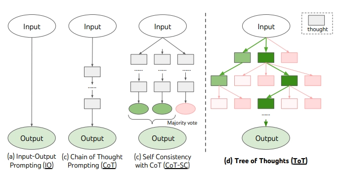
Why do prompt engineering techniques (like CoT) alone hit fundamental limitations when LLMs face problems requiring complex, multi-step reasoning, and what inherent properties of LLMs are related to these limitations?

While prompt engineering techniques like CoT significantly enhance LLMs' complex reasoning capabilities, they hit fundamental limitations due to the following inherent properties of LLMs themselves:
1. Sensitivity to Surface Patterns: LLMs react very sensitively to the surface form of the prompt, such as word choice or sentence structure. Even slight changes in phrasing, while preserving meaning, can lead to unstable results. This is because models rely heavily on statistical pattern learning rather than deep semantic understanding.
2. Limits of Inherent Reasoning Ability: Prompting primarily serves to elicit the reasoning capabilities the model already possesses, rather than creating new logical, mathematical, or common-sense reasoning abilities it lacks. CoT merely makes the model's reasoning process explicit; this process itself can still contain errors. This stems from LLMs learning implicit knowledge and patterns from vast text data, rather than having explicit symbolic manipulation or reasoning engines.
3. Tendency Towards Hallucination: When pushed beyond their knowledge boundaries or faced with very complex reasoning demands, LLMs tend to generate plausible-sounding but factually incorrect or logically inconsistent content (hallucinations). Prompting alone cannot fully guarantee the factual correctness or logical soundness of the generated content.
4. Error Propagation and Difficulty in Correction: In linear step-by-step reasoning methods like CoT, small errors in early steps can propagate and significantly impact the final result. Furthermore, the autoregressive generation process makes it difficult for LLMs to spontaneously correct a flawed reasoning path or explore alternative routes once committed (which ToT aims to mitigate).
5. Context Length Limitation: There's a physical limit to the amount of information (examples, instructions) that can fit into the prompt and the length of the reasoning process (like CoT) that can be represented. Very long and complex problems become intractable with prompting alone.
In conclusion, prompt engineering is a powerful interface for maximizing LLM capabilities, but it cannot overcome the fundamental limitations inherent in the LLM architecture and training paradigm. Achieving breakthroughs in truly complex reasoning likely requires advancements in prompting techniques alongside fundamental improvements in model architecture, learning algorithms, and data strategies.
How can prompts induce planning? Explain frameworks like ReAct for tool use.

Planning behavior can be induced in LLMs by explicitly asking them to create a plan in the prompt. For instance, one could instruct: "First, outline a step-by-step plan to solve this problem, then execute the plan."
The ReAct (Reason + Act) framework provides a more structured approach for enabling LLMs to solve complex tasks by interleaving reasoning and action. It is particularly effective for tasks requiring the use of external tools like search engines, calculators, or API calls.
How ReAct Works:
ReAct typically structures the prompt to make the LLM operate within a thought-action-observation loop:
1. Thought: The LLM considers the current problem state, results from previous steps (observations), and the final goal to analyze the situation and formulate a plan for the next action. (e.g., "I lack current information, I need to search for it.")
2. Action: Based on the plan, the LLM determines the specific action to perform. This usually involves specifying the external tool to use and the input (arguments) for that tool in a defined format. (e.g., Action: Search[keywords to search])
3. Observation: An external system (the ReAct execution environment) actually performs the action specified by the LLM (e.g., calls a search engine API) and obtains the result (e.g., search result summary). This result is provided back as 'observation' information, which is included in the LLM's input prompt for the next cycle.
The LLM repeats this 'Thought → Action → Observation' cycle, dynamically adjusting its plan, leveraging external tools to gather necessary information or perform calculations, and reasoning based on the outcomes. This allows LLMs to effectively tackle complex problems or questions requiring up-to-date information that cannot be solved using their internal knowledge alone.
What core limitations of LLMs do AI agent frameworks like AutoGen or MetaGPT aim to address by leveraging LLMs, and what specific functional components do these frameworks provide to transform LLMs beyond simple text generation tools into goal-oriented problem-solving systems?

AI agent frameworks like AutoGen and MetaGPT build upon the powerful language understanding and generation capabilities of LLMs but are designed to perform complex, multi-step, goal-oriented tasks autonomously, going beyond simple question-answering or text generation. They aim to evolve LLMs from mere 'tools' into 'intelligent agents' capable of planning, acting, interacting, and collaborating.
The core limitations of LLMs that these frameworks seek to address include:
- Lack of State and Memory Management: LLMs can only process information within their limited context window and struggle to maintain long-term state or memory.
- Inability to Interact with the External World: LLMs alone cannot use external tools (APIs, databases, search engines) or interact with real-world environments.
- Limited Complex Planning and Task Decomposition: They lack the ability to systematically create plans and break down complex goals into sub-tasks.
- Poor Self-Reflection and Refinement: Their ability to recognize and correct flaws in their own outputs or plans is limited.
To overcome these limitations, AI agent frameworks use LLMs as their core engine while providing the following functional components:
- Planning and Task Decomposition: Analyze complex user goals to generate and manage plans consisting of sequences or structures of executable sub-tasks.
- Tool Use: Provide interfaces allowing the LLM to call and utilize various external tools as needed, such as APIs, calculators, code interpreters, and search engines (e.g., leveraging the ReAct paradigm).
- Memory Management: Offer long-term memory mechanisms (e.g., using vector databases) that go beyond the short-term context window, allowing agents to store and retrieve information gathered during task execution or from past interactions.
- Multi-Agent Collaboration: Support scenarios where multiple LLM-based agents, potentially with different roles or expertise, can communicate and interact to solve complex problems collaboratively. (e.g., AutoGen's conversational agents, MetaGPT's simulation of role-based software development processes).
- Self-Reflection and Refinement: Enable agents to evaluate their own intermediate outputs (plans, code, documents) and identify/correct issues, thereby improving the quality and reliability of the final results.
In conclusion, AI agent frameworks aim to complement the core capabilities of LLMs by integrating functionalities like planning, tool use, memory, collaboration, and self-reflection. This addresses the limitations of LLMs and seeks to evolve them from simple API endpoints into sophisticated systems capable of tackling complex, practical problems.

IX. Evaluation and Benchmarking

Discuss the challenges in evaluating generative models, contrasting automated metrics with human evaluation.

Evaluating the performance of generative models presents inherent difficulties for several reasons:
Sources of Difficulty:
- Subjectivity and Open-Ended Outputs: Unlike classification or prediction tasks with single correct answers, the quality of generative model outputs (text, images, etc.) can be subjective, and the outputs themselves can be highly diverse. Creativity, style, and aesthetic appeal are hard to quantify.
- Multifaceted Evaluation Criteria: Good generative outputs often need to satisfy multiple criteria simultaneously, such as relevance, factual accuracy, coherence, consistency, fluency, safety, and usefulness. It's difficult for a single metric to capture all these aspects comprehensively.
Comparison of Evaluation Methods:
- Automated Metrics:
  - Examples: BLEU, ROUGE scores for text generation; FID (Fréchet Inception Distance), IS (Inception Score) for image generation.
  - How they work: Typically calculate surface-level features of the output (e.g., word overlap rates, pixel distribution similarity).
  - Pros: Fast, inexpensive, and allow for large-scale evaluation, useful for iterative testing during model development.
  - Cons: Often fail to reflect the actual quality, semantic accuracy, logical errors, creativity, or harmfulness of the generated content accurately. Frequently show low correlation with human preferences.
- Human Evaluation:
  - How it works: Real people directly assess the generated outputs based on predefined criteria (e.g., fluency, relevance, creativity, safety) by assigning scores or comparing preferences.
  - Pros: The most reliable method for assessing aspects missed by automated metrics, such as subtle quality differences, contextual understanding, creativity, and the actual usefulness and safety perceived by users.
  - Cons: Time-consuming, expensive, and labor-intensive. Can suffer from subjectivity, inter-rater disagreement, and potential biases among evaluators. Maintaining evaluation consistency is challenging. In conclusion, there is often a significant gap between what automated metrics can easily measure and what humans actually perceive as high-quality or useful. Therefore, generative model evaluation typically employs both automated metrics and human evaluation in a complementary manner.
How is the intrinsic factuality of LLMs systematically evaluated (e.g., using TruthfulQA)?

Evaluating whether an LLM generates fact-based information or plausibly sounding misinformation (hallucinations) is crucial for its reliability and requires a systematic approach beyond simple accuracy measurement.
Evaluation Methods and Benchmarks:
- Using Specialized Benchmarks:
  - TruthfulQA: Includes questions deliberately designed to mimic common misconceptions or falsehoods that might seem correct. It assesses the model's ability to generate truthful answers instead of merely repeating misinformation it might have learned from the internet.
  - HaluEval: Provides datasets intentionally containing hallucinations to evaluate the model's ability to detect them.
- Measuring Quantitative Metrics:
  - Factual Question Accuracy: Measures how accurately the model answers factual questions with clearly known answers.
  - Faithfulness Evaluation: In RAG systems, assesses how well the model's generated answer aligns with the content of the referenced external documents (context).
  - Calibration Analysis: Analyzes whether the confidence level expressed by the model in its answers correlates well with its actual accuracy. Poor calibration makes it hard to trust the model's outputs.
- Applying Diverse Methodologies:
  - Knowledge Probing: Assesses the extent of the model's knowledge within specific domains.
  - Adversarial Questioning: Uses questions designed to confuse the model or elicit incorrect answers.
  - External Knowledge Verification: Checks claims made by the model against external knowledge bases like Wikipedia or trusted databases.
  - LLM-as-a-Judge: Uses another powerful LLM to evaluate the factuality or quality of the model's answers (though the judge LLM's own biases can interfere).
Systematically evaluating LLM factuality requires using diverse benchmarks and metrics specifically targeting this failure mode (hallucination), often complementing automated scores with careful human analysis.
How is the reasoning ability of LLMs evaluated? Mention key benchmarks.

Evaluating the reasoning ability of LLMs aims to measure higher-order cognitive skills like logical thinking, mathematical problem-solving, step-by-step deduction, and common-sense understanding, going beyond simple information retrieval or pattern memorization. Various benchmarks composed of problems requiring genuine reasoning processes are used for this purpose. Key benchmarks include:
- MMLU (Massive Multitask Language Understanding): Comprehensively evaluates broad knowledge and problem-solving abilities with multiple-choice questions covering 57 diverse subjects, from STEM fields to humanities and social sciences.
- GSM8K (Grade School Math 8K): Consists of grade school level math word problems requiring multiple arithmetic steps, measuring the model's mathematical reasoning and step-by-step problem-solving skills. Often evaluated using Chain-of-Thought (CoT) prompting.
- BIG-Bench (Beyond the Imitation Game Benchmark): A large-scale collaborative benchmark designed to evaluate a wide range of challenging cognitive abilities, including difficult reasoning problems.
- HellaSwag: Assesses commonsense reasoning through multiple-choice questions asking for the most natural continuation of a given context.
- ARC (AI2 Reasoning Challenge): Comprises challenging science questions (elementary and middle school levels) that require reasoning.
- DROP (Discrete Reasoning Over Paragraphs): A reading comprehension benchmark where finding the answer requires additional discrete reasoning steps like addition, counting, or comparison over the provided text.
- MATH: Includes challenging competition-level mathematics problems requiring advanced mathematical reasoning in areas like algebra, geometry, and number theory.
- HumanEval: A benchmark for evaluating code generation ability, which indirectly measures the logical reasoning skills needed to write correct code.
These benchmarks play a crucial role in guiding development towards models with more robust and complex reasoning capabilities, beyond simple memorization or surface pattern matching.
Explain text-to-image model evaluation regarding prompt alignment (CLIP score), quality/realism (FID), and diversity.

Evaluating text-to-image models, which generate images from textual descriptions (prompts), typically involves considering the following three aspects comprehensively:
1. Prompt Alignment and Fidelity:
  - Meaning: Indicates how faithfully the generated image reflects the content and meaning of the input text prompt. It assesses whether the objects, attributes, relationships, and style described in the prompt are well-represented in the image.
  - Key Metric: CLIP Score is widely used. It employs a vision-language model like CLIP to calculate the semantic similarity (e.g., cosine similarity) between the embedding of the input text prompt and the embedding of the generated image. A higher score generally indicates better alignment with the prompt.
2. Image Quality and Realism:
  - Meaning: Evaluates how visually natural and realistic the generated image is, and whether it contains technical flaws.
  - Key Metric: FID (Fréchet Inception Distance) is the standard metric. It uses a pre-trained Inception network to measure the distance between the feature distributions of generated images and real images. A lower FID score indicates that the generated images are statistically more similar to real images, generally implying higher quality and realism.
3. Diversity:
  - Meaning: Refers to the model's ability to generate varied and distinct images for the same or similar prompts. Lack of diversity might indicate 'mode collapse,' where the model repetitively generates only certain types of images.
  - Evaluation: While FID indirectly reflects some diversity, it's not perfect. Often assessed by measuring similarity between generated images, using specific metrics, or frequently through direct human judgment.
Evaluating text-to-image models typically involves combining automated metrics (like CLIP score and FID) with qualitative analysis through human evaluation (assessing aesthetic appeal, accuracy of details, reflection of subtle prompt nuances, etc.) for a comprehensive assessment.
How are multimodal models evaluated? What are the specific challenges?

Evaluating multimodal models, which process multiple types of information (text, image, audio, etc.) simultaneously, is more complex than evaluating unimodal models. It requires measuring not only performance within each modality but also the ability to understand the interactions between modalities and reason based on them.
Evaluation Methods:
- Using Task-Specific Benchmarks: Performance is commonly measured on specific tasks requiring multimodal capabilities.
  - Visual Question Answering (VQA): Assessing the ability to answer questions about an image (e.g., VQAv2, GQA datasets).
  - Image Captioning: Evaluating the ability to generate natural language descriptions for a given image (e.g., COCO Captions dataset, using metrics like BLEU, CIDEr, SPICE).
  - Text-Image Retrieval: Assessing the ability to find images corresponding to text descriptions or vice versa (e.g., Flickr30k, COCO datasets, using Recall@K metric).
  - Other benchmarks exist for video understanding, audio-visual association, etc.
Specific Challenges:
- Verifying True Cross-Modal Reasoning: It's difficult to distinguish whether a model is genuinely integrating information across modalities to reason or just relying on biases or shortcuts within a single modality to arrive at the correct answer.
- Evaluating Cross-Modal Consistency: For instance, if a model generates both an image and its description, automatically assessing whether the generated text accurately and consistently describes the generated image is challenging.
- Lack of Reasoning Process Evaluation: Standardized methodologies are lacking for evaluating the validity of the cross-modal reasoning process itself that leads to the final output, beyond just checking the correctness of the final answer.
- Data Scarcity: Large-scale, high-quality benchmark data specifically designed to evaluate complex multimodal reasoning capabilities is often still insufficient.
- Subjectivity and Reliance on Human Evaluation: Judging the quality, relevance, and creativity of generated multimodal content inherently involves subjectivity, often necessitating carefully designed human evaluation for reliable assessment.
What are the known limitations or 'gaming' issues with generative model benchmarks?

While benchmarks are essential tools for measuring progress and comparing generative models, they suffer from well-known limitations and potential issues (sometimes called 'gaming' or 'benchmark hacking'):
- Data Contamination: When the test set data, intended for evaluation, unintentionally gets included in the model's pre-training data. In such cases, the model achieves artificially high scores by simply 'memorizing' the answers, invalidating fair performance comparison. This is prone to happen with large web-scraped datasets.
- Benchmark Overfitting: The phenomenon where models become overly optimized for the specific format, question types, or data distribution of the benchmark itself. This can lead to high benchmark scores but poor generalization to real-world, diverse problems.
- Gap Between Metrics and Real Performance: As mentioned earlier, high scores on automated metrics like BLEU or FID do not necessarily guarantee high perceived quality, usefulness, creativity, or safety by humans.
- Sensitivity to Evaluation Setup: Model performance can vary significantly depending on the specific prompts used, sampling parameters applied, etc. Inconsistent or unreported evaluation conditions make direct model comparison difficult.
- Benchmark Staleness and Saturation: Most benchmarks remain static once created. As models improve over time, benchmark tasks can become too easy ('solved'), losing their ability to differentiate the performance of state-of-the-art models.
- Evaluator Bias: Evaluation methods relying on human judgment or LLM-as-a-judge are susceptible to subjectivity, preconceptions, lack of consistency, and other biases of the evaluators.
Due to these limitations, benchmark scores should always be interpreted critically and ideally supplemented with qualitative analysis, additional human evaluations, and tests in real-world application settings for a comprehensive judgment of model performance.
What are techniques for interpreting Transformer behavior (e.g., attention visualization, feature attribution)?

Understanding why a Transformer model makes a specific prediction or generates a certain output – i.e., understanding its internal workings – is crucial for debugging, building trust, improving performance, and ensuring safety. Various interpretation techniques are used for this purpose:
- Attention Visualization:
  - Method: Visualizing the attention weights calculated in the model's attention layers to see which other tokens in the input sequence a particular token 'attended' to more strongly when generating a prediction.
  - Limitation: Research suggests that high attention weights do not always equate to high importance of the attended token.
- Feature Attribution / Importance Analysis (Saliency):
  - Method: Aims to quantify how much each input feature (e.g., a specific word token) contributed to or was important for the model's final output (e.g., a specific prediction probability).
  - Technique Examples: Gradient-based methods that use gradients of the output with respect to the input (e.g., Integrated Gradients), and perturbation-based methods that observe output changes when parts of the input are modified (e.g., LIME).
- Probing Internal Activations:
  - Method: Analyzing the activation patterns of specific neurons or layers inside the model to investigate if they correlate with specific linguistic properties (e.g., part-of-speech, syntactic structure), concepts, or task-related features.
  - Recent Trend: Active research using Sparse AutoEncoders (SAEs) to extract interpretable, sparse features from high-dimensional activation vectors.
- Mechanistic Interpretability:
  - Method: A very ambitious approach that aims to reverse-engineer the actual algorithms or 'circuits' the model has learned to perform specific tasks by meticulously analyzing how its weights and individual components (attention heads, MLP layers, etc.) interact.
- Ablation Studies:
  - Method: Systematically removing or disabling parts of the model (e.g., specific attention heads, certain layers) and observing the resulting change in performance to understand the function or importance of the ablated component.
These interpretation techniques each have their strengths and weaknesses. Relying on a single method is often insufficient; combining multiple techniques usually provides deeper and more comprehensive insights into model behavior.

Appendix: Recommended Learning Resources

Transformer Basics
Advanced LLM Architectures and Concepts
- A Visual Guide to Mixture of Experts(MoE)
- Mixture of Experts Explained
Advanced Training and Fine-tuning Techniques
Multimodal Models
- Multimodality and Large Multimodal Models (LMMs)
- Understanding Multimodal LLMs
Image Generation and Diffusion Models
- The Illustrated Stable Diffusion
- What are Diffusion Models?
Foundation Model Engineering and Infrastructure
- A Visual Guide to Quantization
Reasoning, Prompting, and Agents