


![[The AI Show Episode 145]: OpenAI Releases o3 and o4-mini, AI Is Causing “Quiet Layoffs,” Executive Order on Youth AI Education & GPT-4o’s Controversial Update](https://www.marketingaiinstitute.com/hubfs/ep%20145%20cover.png)


_NicoElNino_Alamy.jpg?width=1280&auto=webp&quality=80&disable=upscale#)


![Standalone Meta AI App Released for iPhone [Download]](https://www.iclarified.com/images/news/97157/97157/97157-640.jpg)


Graph Neural Networks Part 4: Teaching Models to Connect the Dots
Heuristic and GNN-based approaches to Link Prediction The post Graph Neural Networks Part 4: Teaching Models to Connect the Dots appeared first on Towards Data Science.

Link prediction is a very popular topic! It can be used to recommend friends in social networks, suggest products on e-commerce sites or movies on Netflix, or predict protein interactions in biology. In this post, you will explore how link prediction works. First you will learn simple heuristics, and we end with powerful GNN-based methods like SEAL.
The previous posts explained GCNs, GATs, and GraphSage. They mainly covered predicting node properties, so you can read this article standalone, because this time we shift focus to predicting edges. If you want to dive a bit deeper into node representations, I recommend to revisit the previous posts. The code setup can be found here.
What is Link Prediction?
Link prediction is the task of forecasting missing or future connections (edges) between nodes in a graph. Given a graph G = (V, E), the goal is to predict whether an edge should exist between two nodes (u, v) ∉ E.
To evaluate link prediction models, you can create a test set by hiding a portion of the existing edges and ask the model to predict them. Of course, the test set should have positive samples (real edges), and negative samples (random node pairs that are not connected). You can train the model on the remaining graph.
The output of the model is a link score or probability for each node pair. You can evaluate this with metrics like AUC or average precision.
We will take a look at simple heuristic-based methods, and then we move on to more complex methods.

Heuristic-Based Methods
We can divide these ‘easy’ methods into two categories: local and global. Local heuristics are based on local structure, while global heuristics use the whole graph. These approaches are rule-based and work well as baselines for link prediction tasks.
Local Heuristics
As the name says, local heuristics rely on the immediate neighborhood of the two nodes you are testing for a potential link. And actually they can be surprisingly effective. Benefits of local heuristics are that they are fast and interpretable. But they only look at the close neighborhood, so capturing the complexity of relationships is limited.
Common Neighbors
The idea is simple: if two nodes share many common neighbors, they are more likely to be connected.
For calculation you count the number of neighbors the nodes have in common. One issue here is that it does not take into account the relative number of common neighbors.
In the examples below, the number of common neighbors between A and B is 3, and the number of common neighbors between C and D is 1.

Jaccard Coefficient
The Jaccard Coefficient fixes the issue of common neighbors and computes the relative number of neighbors in common.
You take the common neighbors and divide this by the total number of unique neighbors of the two nodes.
So now things change a bit: the Jaccard coefficient of nodes A and B is 3/5 = 0.6 (they have 3 common neighbors and 5 total unique neighbors), while the Jaccard coefficient of nodes C and D is 1/1 = 1 (they have 1 common neighbor and 1 unique neighbor). In this case the connection between C and D is more likely, because they only have 1 neighbor, and it’s also a common neighbor.

Adamic-Adar Index
The Adamic-Adar index goes one step further than common neighbors: it uses the popularity of a common neighbor and gives less weight to more popular neighbors (they have more connections). The intuition behind this is that if a node is connected to everyone, it doesn’t tell us much about a specific connection.
What does that look like in a formula?

So for each common neighbor z, we add a score of 1 divided by the log of the number of neighbors from z. By doing this, the more popular the common neighbor, the smaller its contribution.
Let’s calculate the Adamic-Adar index for our examples.

Preferential Attachment
A different approach is preferential attachment. The idea behind it is that nodes with higher degrees are more likely to form links. Calculation is super easy, you just multiply the degrees (number of connections) of the two nodes.
For A and B, the degrees are respectively 5 and 3, so the score is 5*3 = 15. C and D have a score of 1*1 = 1. In this case A and B are more likely to have a connection, because they have more neighbors in general.

Global Heuristics
Global heuristics consider paths, walks, or the entire graph structure. They can capture richer patterns, but are more computationally expensive.
Katz Index
The most well-known global heuristic for Link Prediction is the Katz Index. It takes all the different paths between two nodes (usually only paths up to three steps). Each path gets a weight that decays exponentially with its length. This makes sense intuitively, because the shorter a path, the more important it is (friends in common means a lot). On the other hand, indirect paths matter as well! They can hint at potential links.
The Katz Formula:

We take two nodes, C and E, and count the paths between them. There are three paths with up to three steps: one path with two steps (orange), and two paths with three steps (blue and green). Now we can calculate the Katz index, let’s choose 0.1 for beta:

Rooted PageRank
This method uses random walks to determine how likely it is that a random walk from the first node, will end up in the second node. So you start in the first node, then you either walk to a random neighbor, or you jump back to the first node. The probability that you end up at the second node tells how closely the two nodes are. If the probability is high, there is a good chance the nodes should be linked.
ML-Based Link Prediction
Machine learning approaches take link prediction beyond heuristics by learning patterns directly from the data. Instead of relying on predefined rules, ML models can learn complex features that signal whether a link should exist.
A basic approach is to treat link prediction as a binary classification task: for each node pair (u, v), we create a feature vector and train a model to predict 1 (link exists) or 0 (link doesn’t exist). You can add the heuristics we calculated before as features. The heuristics didn’t agree all the time on likelihood of edges, sometimes the edge between A and B was more likely, while for others the edge between C and D was the better choice. By including multiple scores as features we don’t have to choose one heuristic. Of course depending on the problem some heuristics might work better than others.
Another type of features you can add are aggregated features: for example node degree, node embeddings, attribute averages, etc.
Then use any classifier (e.g., logistic regression, random forest, XGBoost) to predict links. This already performs better than heuristics alone, especially when combined.
In this post we will use the Cora dataset to test different approaches to link prediction. The Cora dataset contains scientific papers. The edges represent citations between papers. Let’s train a machine learning model as baseline, where we only add the Jaccard coefficient:
import os.path as osp

from sklearn.linear_model import LogisticRegression
from sklearn.metrics import roc_auc_score, average_precision_score
from torch_geometric.datasets import Planetoid
from torch_geometric.transforms import RandomLinkSplit
from torch_geometric.utils import to_dense_adj

# reproducibility
from torch_geometric import seed_everything
seed_everything(42)

# load Cora dataset, create train/val/test splits
path = osp.join(osp.dirname(osp.realpath(__file__)), '..', 'data', 'Planetoid')
dataset = Planetoid(path, name='Cora')

data_all = dataset[0]
transform = RandomLinkSplit(num_val=0.05, num_test=0.1, is_undirected=True, split_labels=True)
train_data, val_data, test_data = transform(data_all)

# add Jaccard and train with Logistic Regression
adj = to_dense_adj(train_data.edge_index, max_num_nodes=data_all.num_nodes)[0]

def jaccard(u, v, adj):
    u_neighbors = set(adj[u].nonzero().view(-1).tolist())
    v_neighbors = set(adj[v].nonzero().view(-1).tolist())
    inter = len(u_neighbors & v_neighbors)
    union = len(u_neighbors | v_neighbors)
    return inter / union if union > 0 else 0.0

def extract_features(pairs, adj):
    return [[jaccard(u, v, adj)] for u, v in pairs]

train_pairs = train_data.pos_edge_label_index.t().tolist() + train_data.neg_edge_label_index.t().tolist()
train_labels = [1] * train_data.pos_edge_label_index.size(1) + [0] * train_data.neg_edge_label_index.size(1)

test_pairs = test_data.pos_edge_label_index.t().tolist() + test_data.neg_edge_label_index.t().tolist()
test_labels = [1] * test_data.pos_edge_label_index.size(1) + [0] * test_data.neg_edge_label_index.size(1)

X_train = extract_features(train_pairs, adj)
clf = LogisticRegression().fit(X_train, train_labels)

X_test = extract_features(test_pairs, adj)
probs = clf.predict_proba(X_test)[:, 1]
auc_ml = roc_auc_score(test_labels, probs)
ap_ml = average_precision_score(test_labels, probs)
print(f"[ML Heuristic] AUC: {auc_ml:.4f}, AP: {ap_ml:.4f}")
We evaluate with AUC. This is the result:
[ML Model] AUC: 0.6958, AP: 0.6890We can go a step further and use neural networks that operate directly on the graph structure.
VGAE: Encoding and Decoding
A Variational Graph Auto-Encoder is like a neural network that learns to guess the hidden structure of the graph. It can then use that hidden knowledge to predict missing links.
A VGAE is actually a combination of a GAE (Graph Auto-Encoder) and a VAE (Variational Auto-Encoder). I’ll get back to the difference between a GAE and a VGAE later on.
The steps of a VGAE are as follows. First, the VGAE encodes nodes into latent vectors, and then it decodes node pairs to predict whether an edge exists between them.
How does the encoding work? Each node is mapped to a latent variable, that is a point in some hidden space. The encoder is a Graph Convolutional Network (GCN) that produces a mean and a variance vector for each node. It uses the node features and the adjacency matrix as input. Using the vectors, the VGAE samples a latent embedding from a normal distribution. It’s important to note that each node isn’t just mapped to a single point, but to a distribution! This is the difference between a GAE and a VGAE, in a GAE each node is mapped to one single point.

The next step is the decoding step. The VGAE will guess if there is an edge between two nodes. It does this by calculating the inner product between the embeddings of the two nodes:

The thought behind it is: if the nodes are closer together in the hidden space, it’s more likely they are connected.
VGAE visualized:

How does the model learn? It optimizes two things:
- Reconstruction Loss: Do the predicted edges match the real ones?
- KL Divergence Loss: Is the latent space nice and regular?
Let’s test the VGAE on the Cora dataset:
import os.path as osp

import numpy as np
import torch
from sklearn.metrics import roc_auc_score, average_precision_score

from torch_geometric.datasets import Planetoid
from torch_geometric.nn import GCNConv, VGAE
from torch_geometric.transforms import RandomLinkSplit

# same as before
from torch_geometric import seed_everything
seed_everything(42)

path = osp.join(osp.dirname(osp.realpath(__file__)), '..', 'data', 'Planetoid')
dataset = Planetoid(path, name='Cora')

data_all = dataset[0]
transform = RandomLinkSplit(num_val=0.05, num_test=0.1, is_undirected=True, split_labels=True)
train_data, val_data, test_data = transform(data_all)

# VGAE
class VGAEEncoder(torch.nn.Module):
    def __init__(self, in_channels, out_channels):
        super().__init__()
        self.conv1 = GCNConv(in_channels, 2 * out_channels)
        self.conv_mu = GCNConv(2 * out_channels, out_channels)
        self.conv_logstd = GCNConv(2 * out_channels, out_channels)

    def forward(self, x, edge_index):
        x = self.conv1(x, edge_index).relu()
        return self.conv_mu(x, edge_index), self.conv_logstd(x, edge_index)

vgae = VGAE(VGAEEncoder(dataset.num_features, 32))
vgae_optimizer = torch.optim.Adam(vgae.parameters(), lr=0.01)

x = data_all.x
edge_index = train_data.edge_index

# train VGAE model
for epoch in range(1, 101):
    vgae.train()
    vgae_optimizer.zero_grad()
    z = vgae.encode(x, edge_index)
    # reconstruction loss
    loss = vgae.recon_loss(z, train_data.pos_edge_label_index)
    # KL divergence
    loss = loss + (1 / data_all.num_nodes) * vgae.kl_loss()
    loss.backward()
    vgae_optimizer.step()

vgae.eval()
z = vgae.encode(x, edge_index)

@torch.no_grad()
def score_edges(pairs):
    edge_tensor = torch.tensor(pairs).t().to(z.device)
    return vgae.decoder(z, edge_tensor).view(-1).cpu().numpy()

vgae_scores = np.concatenate([score_edges(test_data.pos_edge_label_index.t().tolist()),
                              score_edges(test_data.neg_edge_label_index.t().tolist())])
vgae_labels = np.array([1] * test_data.pos_edge_label_index.size(1) +
                       [0] * test_data.neg_edge_label_index.size(1))

auc_vgae = roc_auc_score(vgae_labels, vgae_scores)
ap_vgae = average_precision_score(vgae_labels, vgae_scores)
print(f"[VGAE] AUC: {auc_vgae:.4f}, AP: {ap_vgae:.4f}")
And the result (ML model added for comparison):
[VGAE]     AUC: 0.9032, AP: 0.9179
[ML Model] AUC: 0.6958, AP: 0.6890
Wow! Massive improvement compared to the ML model!
SEAL: Learning from Subgraphs
One of the most powerful GNN-based approaches is SEAL (Subgraph Embedding-based Link prediction). The idea is simple and elegant: instead of looking at global node embeddings, SEAL looks at the local subgraph around each node pair.
Here’s a step by step explanation:
- For each node pair (u, v), extract a small enclosing subgraph. E.g., neighbors only (1-hop neighborhood) or neighbors and neighbors from neighbors (2-hop neighborhood).
- Label the nodes in this subgraph to reflect their role: which ones are u, v, and which ones are neighbors.
- Use a GNN (like DGCNN or GCN) to learn from the subgraph and predict if a link should exist.
Visualization of the steps:

SEAL is very powerful because it learns structural patterns directly from examples, instead of relying on handcrafted rules. It also works well with sparse graphs and generalizes across different types of networks.
Let’s see if SEAL can improve the results of the VGAE on the Cora dataset. For the SEAL code, I took the sample code from PyTorch geometric (check it out by following the link), since SEAL requires quite some processing. You can recognize the different steps in the code (preparing the data, extracting the subgraphs, labeling the nodes). Training for 50 epochs gives the following result:
[SEAL]     AUC: 0.9038, AP: 0.9176
[VGAE]     AUC: 0.9032, AP: 0.9179
[ML Model] AUC: 0.6958, AP: 0.6890
Almost exactly the same result as the VGAE. So for this problem, VGAE might be the best choice (VGAE is significantly faster than SEAL). Of course this can vary, depending on your problem.
Conclusion
In this post, we dived into the topic of link prediction, from heuristics to SEAL. Heuristic methods are fast and interpretable and can serve as good baselines, but ML and GNN-based methods like VGAE and SEAL can learn richer representations and offer better performance. Depending on your dataset size and task complexity, it’s worth exploring both!
Thanks for reading, until next time!
Related
Graph Neural Networks Part 1. Graph Convolutional Networks Explained
Graph Neural Networks Part 2. Graph Attention Networks vs. GCNs
Graph Neural Networks Part 3: How GraphSAGE Handles Changing Graph Structure
The post Graph Neural Networks Part 4: Teaching Models to Connect the Dots appeared first on Towards Data Science.


