Comparing Optimization Algorithms: Lessons from the Himmelblau Function

Optimization algorithms are the unsung heroes behind many computational tasks, from training machine learning models to solving engineering problems. A recent paper, A Comparative Analysis of Optimization Algorithms: The Himmelblau Function Case Study (April 22, 2025), dives into how four algorithms tackle the Himmelblau function, a tricky test problem with multiple solutions. This article distills the study’s core findings for developers, keeping the technical details intact but simple and math-free. What’s the Himmelblau Function? The Himmelblau function is a benchmark problem used to test optimization algorithms. It’s like a hilly landscape with four identical “valleys” (global minima) where the best solutions lie, plus some deceptive “shallow dips” (local minima) that can trap algorithms. Its complexity makes it perfect for comparing how well algorithms find the true valleys versus getting stuck. The Algorithms Tested The study compares four optimization algorithms, each run 360 times on the Himmelblau function: SA_Noise: Simulated Annealing with added randomness to explore more of the landscape. SA_T10: Simulated Annealing with a fixed “temperature” of 10, controlling how much it explores versus exploits. Hybrid_SA_Adam: A mix of Simulated Annealing and the Adam optimizer, blending exploration with precise steps. Adam_lr0.01: The Adam optimizer with a learning rate of 0.01, a popular choice in machine learning for steady progress. How They Were Judged Performance was measured by: Steps to converge: How many iterations it took to settle on a solution. Final loss: How close the solution’s value was to zero (the ideal value for the Himmelblau function’s valleys). Success rate: The percentage of runs with a final loss below 1.0 (close enough to a valley). Consistency: Confidence intervals for steps, loss, and distance to the nearest valley, showing how reliable each algorithm was. Key Results Across all runs, the algorithms averaged 238.73 steps, a final loss of 0.52, and an 81.11% success rate. But each algorithm had its own strengths and weaknesses: Steps to Converge SA_Noise and SA_T10: Super fast, needing about 52–62 steps on average. They’re like sprinters, rushing to a solution. Hybrid_SA_Adam: Slower, taking 194–208 steps, balancing speed and caution. Adam_lr0.01: The slowest, requiring 585–693 steps, as it methodically inches toward the best solution. Final Loss Hybrid_SA_Adam and Adam_lr0.01: Nailed it, hitting near-zero loss (0.00–0.00), meaning they consistently found the true valleys. SA_Noise and SA_T10: Less precise, with losses of 0.69–1.38 and 0.87–1.38, often landing in shallow dips instead of valleys. Distance to the True Solution All algorithms ended up about 4.05–4.41 units from the nearest valley, but Hybrid_SA_Adam had the tightest range (4.08–4.28), showing precision. Visual Insights Boxplots: Showed SA_Noise and SA_T10 as fast but sloppy, while Hybrid_SA_Adam and Adam_lr0.01 were slower but spot-on. Convergence Plot: Adam_lr0.01 dropped to near-zero loss in just 200 steps, outpacing others in accuracy. Heatmap of Failures: SA_T10 struggled most, racking up high losses when stuck about 4.0 units from a valley. Metric Overall Value Number of Runs 360 Average Steps 238.73 Average Final Loss 0.52 Success Rate (

May 5, 2025 - 05:29

Comparing Optimization Algorithms: Lessons from the Himmelblau Function

Optimization algorithms are the unsung heroes behind many computational tasks, from training machine learning models to solving engineering problems. A recent paper, A Comparative Analysis of Optimization Algorithms: The Himmelblau Function Case Study (April 22, 2025), dives into how four algorithms tackle the Himmelblau function, a tricky test problem with multiple solutions. This article distills the study’s core findings for developers, keeping the technical details intact but simple and math-free.

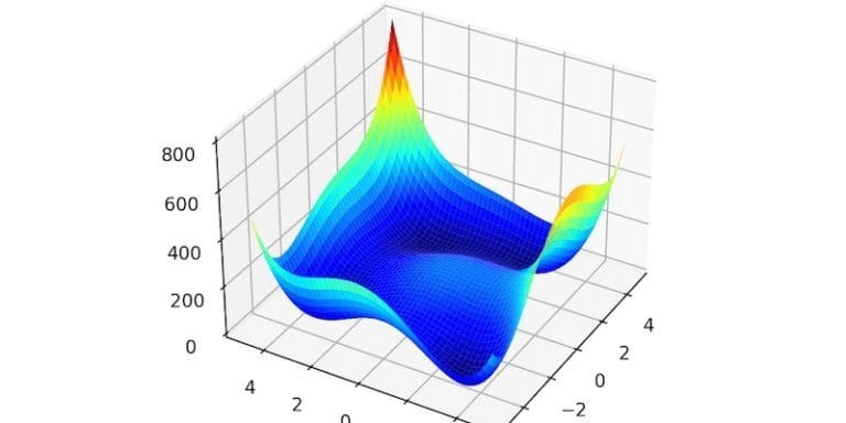
What’s the Himmelblau Function?

The Himmelblau function is a benchmark problem used to test optimization algorithms. It’s like a hilly landscape with four identical “valleys” (global minima) where the best solutions lie, plus some deceptive “shallow dips” (local minima) that can trap algorithms. Its complexity makes it perfect for comparing how well algorithms find the true valleys versus getting stuck.

The Algorithms Tested

The study compares four optimization algorithms, each run 360 times on the Himmelblau function:

SA_Noise: Simulated Annealing with added randomness to explore more of the landscape.

SA_T10: Simulated Annealing with a fixed “temperature” of 10, controlling how much it explores versus exploits.

Hybrid_SA_Adam: A mix of Simulated Annealing and the Adam optimizer, blending exploration with precise steps.

Adam_lr0.01: The Adam optimizer with a learning rate of 0.01, a popular choice in machine learning for steady progress.

How They Were Judged

Performance was measured by:

Steps to converge: How many iterations it took to settle on a solution.

Final loss: How close the solution’s value was to zero (the ideal value for the Himmelblau function’s valleys).

Success rate: The percentage of runs with a final loss below 1.0 (close enough to a valley).

Consistency: Confidence intervals for steps, loss, and distance to the nearest valley, showing how reliable each algorithm was.

Key Results

Across all runs, the algorithms averaged 238.73 steps, a final loss of 0.52, and an 81.11% success rate. But each algorithm had its own strengths and weaknesses:

Steps to Converge

SA_Noise and SA_T10: Super fast, needing about 52–62 steps on average. They’re like sprinters, rushing to a solution.

Hybrid_SA_Adam: Slower, taking 194–208 steps, balancing speed and caution.

Adam_lr0.01: The slowest, requiring 585–693 steps, as it methodically inches toward the best solution.

Final Loss

Hybrid_SA_Adam and Adam_lr0.01: Nailed it, hitting near-zero loss (0.00–0.00), meaning they consistently found the true valleys.

SA_Noise and SA_T10: Less precise, with losses of 0.69–1.38 and 0.87–1.38, often landing in shallow dips instead of valleys.

Distance to the True Solution

All algorithms ended up about 4.05–4.41 units from the nearest valley, but Hybrid_SA_Adam had the tightest range (4.08–4.28), showing precision.

Visual Insights

Boxplots: Showed SA_Noise and SA_T10 as fast but sloppy, while Hybrid_SA_Adam and Adam_lr0.01 were slower but spot-on.

Convergence Plot: Adam_lr0.01 dropped to near-zero loss in just 200 steps, outpacing others in accuracy.

Heatmap of Failures: SA_T10 struggled most, racking up high losses when stuck about 4.0 units from a valley.

Metric

Overall Value

Number of Runs

360

Average Steps

238.73

Average Final Loss

0.52

Success Rate (<1.0)

81.11%

What This Means for Devs

The study reveals a classic trade-off: speed versus accuracy.

Need speed? SA_Noise and SA_T10 are your go-to for quick results, like in real-time systems where a “good enough” solution works.

Need precision? Hybrid_SA_Adam and Adam_lr0.01 shine for tasks like machine learning, where finding the absolute best solution matters.

Mix and match: The hybrid approach shows combining algorithms can balance exploration (finding new areas) and exploitation (honing in on the best spot).

Why It’s Cool

For developers, this study is a playbook for picking the right tool for the job:

Algorithm choice matters: Different problems need different strategies. The Himmelblau function’s multiple valleys mimic real-world challenges like neural network training or resource allocation.

Experimentation is key: Running 360 tests per algorithm gave clear insights into reliability, something you can replicate in your projects.

Visuals help: Boxplots and heatmaps make it easier to spot patterns, so use them to debug or compare your own algorithms.

Try It Out

Want to test an optimizer? Here’s a Python snippet using Adam to minimize a simple function (not Himmelblau, but you get the idea). Tweak it for the Himmelblau function by swapping the loss function.

import tensorflow as tf import numpy as np import matplotlib.pyplot as plt

Simple loss function (replace with Himmelblau for real test)

def loss_function(x): return tf.reduce_sum(x**2) # Minimize x^2 + y^2

Initialize variables

x = tf.Variable([1.0, 1.0], dtype=tf.float32) optimizer = tf.keras.optimizers.Adam(learning_rate=0.01) steps = 200 losses = []

Optimization loop

for step in range(steps): with tf.GradientTape() as tape: loss = loss_function(x) gradients = tape.gradient(loss, [x]) optimizer.apply_gradients(zip(gradients, [x])) losses.append(loss.numpy())

Plot convergence

plt.plot(losses) plt.xlabel('Step') plt.ylabel('Loss') plt.title('Adam Optimization') plt.savefig('adam_convergence.png')
The notebook: https://www.kaggle.com/datasets/allanwandia/himmelblau