Solving the Navier-Stokes Equation with Physics-Informed Neural Networks: A New Frontier in CFD

The Navier-Stokes equations are the backbone of fluid dynamics, describing how liquids and gases move. Solving them is tough, especially for complex flows like turbulence, because they’re nonlinear and chaotic. A new paper, Physics-Informed Neural Networks for Solving the Navier-Stokes Equation: Preliminary Results (April 2025), introduces a way to tackle this using Physics-Informed Neural Networks (PINNs). This article breaks down the core ideas for developers, keeping the technical essence without heavy math. Why Navier-Stokes Is Hard The Navier-Stokes equations model fluid velocity and pressure, ensuring the flow is incompressible (no net gain or loss of fluid in a given space). Traditional solvers, like direct numerical simulation, are slow and resource-heavy, especially for turbulent flows with tiny, chaotic details. PINNs offer a faster, smarter alternative by blending machine learning with the physics of the equations. How PINNs Work PINNs are neural networks that predict fluid properties—velocity (how fast the fluid moves in x and y directions) and pressure—based on time and spatial coordinates. What makes them special is their loss function, which includes: Data loss: How well predictions match known data. Physics loss: How well predictions follow the Navier-Stokes rules and incompressibility. Regularization: A tweak to prevent overfitting. This setup lets PINNs learn from both data and physics, needing less data than traditional machine learning models. The Setup The study trains a feedforward neural network on a dataset of simulated laminar (smooth) fluid flows. It runs for 50 epochs using the Adam optimizer, with early stopping to avoid overfitting. Training happens on a GPU, with data prep on the CPU. The model’s performance is checked via: Training/validation loss: How well it learns overall. Velocity/pressure accuracy: How close predictions are to true fluid behavior. What They Found Learning Performance The training loss drops from 50 to 25 over 30 epochs, showing the PINN learns the physics well. Validation loss settles at 4.9, meaning it generalizes to new data. The gap between training and validation loss suggests the model leans heavily on physics rules, which is good but may miss some data nuances. Fluid Behavior The PINN predicts velocity and pressure fields decently but struggles with details: X-velocity: Captures the range (-0.4 to 0.8) but misses the full true range (-0.4 to 1.2), smoothing out small variations. Y-velocity: Predicts a narrower range (-0.4 to 0.2) than the true (-0.4 to 0.4), which could mess with incompressibility. Pressure: Predicts -3.5 to 0, far from the true -7 to 0, showing it’s hard to nail pressure gradients. Metric Value Final Training Loss 25.0 Final Validation Loss 4.9 Predicted X-Velocity -0.4 to 0.8 True X-Velocity -0.4 to 1.2 Predicted Y-Velocity -0.4 to 0.2 True Y-Velocity -0.4 to 0.4 Predicted Pressure -3.5 to 0 True Pressure -7 to 0 Why It Matters for Devs PINNs are a game-changer for developers working on physics-driven problems: Less Data Needed: By baking physics into the model, PINNs work with smaller datasets, unlike purely data-driven models. Flexible Framework: The approach can apply to other physics problems, like heat or electromagnetism. Room for Innovation: The model’s limits (e.g., missing fine details) point to opportunities for better architectures. What’s Next The researchers plan to level up by: Mixing Models: Combining PINNs with convolutional or recurrent networks to better handle spatial and temporal patterns. Auto-Tuning: Using tools like Optuna to optimize hyperparameters automatically. Tackling Turbulence: Building ensemble models to handle chaotic, turbulent flows. These steps aim to fix the model’s weaknesses, like capturing small-scale fluid details and accurate pressure. Try It Yourself Want to play with PINNs? Here’s a simple Python snippet to get started with a basic neural network in TensorFlow. It’s not the full Navier-Stokes solver but shows the idea: import tensorflow as tf import numpy as np # Simple PINN model class PINN(tf.keras.Model): def init(self): super(PINN, self).init() self.layers = [tf.keras.layers.Dense(50, activation='tanh') for _ in range(3)] self.output = tf.keras.layers.Dense(2) # Predict velocity, pressure def call(self, inputs): x = inputs for layer in self.layers: x = layer(x) return self.output(x) # Fake data (x, t coordinates) x = np.linspace(0, 1, 100).reshape(-1, 1) t = np.linspace(0, 1, 100).reshape(-1, 1) inputs = np.stack([x.flatten(), t.flatten()], axis=1).astype(np.float32) # Setup model model = PINN() optimizer = tf.keras.optimizers.Adam(0.001) model.compile(optimizer=optimizer, loss='mse') # Basic training @tf.function def train_step(inputs):

Apr 28, 2025 - 05:17

Solving the Navier-Stokes Equation with Physics-Informed Neural Networks: A New Frontier in CFD

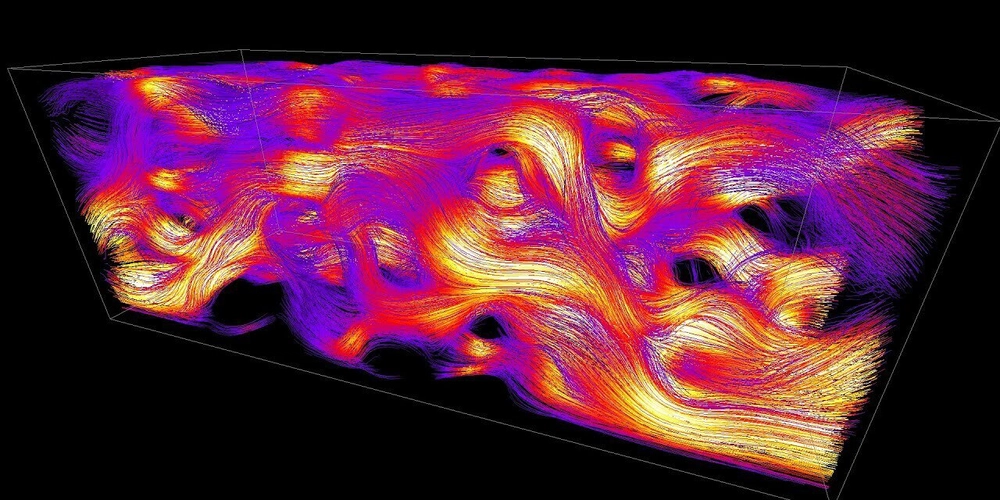
The Navier-Stokes equations are the backbone of fluid dynamics, describing how liquids and gases move. Solving them is tough, especially for complex flows like turbulence, because they’re nonlinear and chaotic. A new paper, Physics-Informed Neural Networks for Solving the Navier-Stokes Equation: Preliminary Results (April 2025), introduces a way to tackle this using Physics-Informed Neural Networks (PINNs). This article breaks down the core ideas for developers, keeping the technical essence without heavy math.

Why Navier-Stokes Is Hard

The Navier-Stokes equations model fluid velocity and pressure, ensuring the flow is incompressible (no net gain or loss of fluid in a given space). Traditional solvers, like direct numerical simulation, are slow and resource-heavy, especially for turbulent flows with tiny, chaotic details. PINNs offer a faster, smarter alternative by blending machine learning with the physics of the equations.

How PINNs Work

PINNs are neural networks that predict fluid properties—velocity (how fast the fluid moves in x and y directions) and pressure—based on time and spatial coordinates. What makes them special is their loss function, which includes:

Data loss: How well predictions match known data.
Physics loss: How well predictions follow the Navier-Stokes rules and incompressibility.
Regularization: A tweak to prevent overfitting.

This setup lets PINNs learn from both data and physics, needing less data than traditional machine learning models.

The Setup

The study trains a feedforward neural network on a dataset of simulated laminar (smooth) fluid flows. It runs for 50 epochs using the Adam optimizer, with early stopping to avoid overfitting. Training happens on a GPU, with data prep on the CPU. The model’s performance is checked via:

Training/validation loss: How well it learns overall.
Velocity/pressure accuracy: How close predictions are to true fluid behavior.

What They Found

Learning Performance

The training loss drops from 50 to 25 over 30 epochs, showing the PINN learns the physics well. Validation loss settles at 4.9, meaning it generalizes to new data. The gap between training and validation loss suggests the model leans heavily on physics rules, which is good but may miss some data nuances.

Fluid Behavior

The PINN predicts velocity and pressure fields decently but struggles with details:

X-velocity: Captures the range (-0.4 to 0.8) but misses the full true range (-0.4 to 1.2), smoothing out small variations.
Y-velocity: Predicts a narrower range (-0.4 to 0.2) than the true (-0.4 to 0.4), which could mess with incompressibility.
Pressure: Predicts -3.5 to 0, far from the true -7 to 0, showing it’s hard to nail pressure gradients.

Metric	Value
Final Training Loss	25.0
Final Validation Loss	4.9
Predicted X-Velocity	-0.4 to 0.8
True X-Velocity	-0.4 to 1.2
Predicted Y-Velocity	-0.4 to 0.2
True Y-Velocity	-0.4 to 0.4
Predicted Pressure	-3.5 to 0
True Pressure	-7 to 0

Why It Matters for Devs

PINNs are a game-changer for developers working on physics-driven problems:

Less Data Needed: By baking physics into the model, PINNs work with smaller datasets, unlike purely data-driven models.
Flexible Framework: The approach can apply to other physics problems, like heat or electromagnetism.
Room for Innovation: The model’s limits (e.g., missing fine details) point to opportunities for better architectures.

What’s Next

The researchers plan to level up by:

Mixing Models: Combining PINNs with convolutional or recurrent networks to better handle spatial and temporal patterns.
Auto-Tuning: Using tools like Optuna to optimize hyperparameters automatically.
Tackling Turbulence: Building ensemble models to handle chaotic, turbulent flows.

These steps aim to fix the model’s weaknesses, like capturing small-scale fluid details and accurate pressure.

Try It Yourself

Want to play with PINNs? Here’s a simple Python snippet to get started with a basic neural network in TensorFlow. It’s not the full Navier-Stokes solver but shows the idea:

import tensorflow as tf
import numpy as np

# Simple PINN model
class PINN(tf.keras.Model):
    def __init__(self):
        super(PINN, self).__init__()
        self.layers = [tf.keras.layers.Dense(50, activation='tanh') for _ in range(3)]
        self.output = tf.keras.layers.Dense(2)  # Predict velocity, pressure

    def call(self, inputs):
        x = inputs
        for layer in self.layers:
            x = layer(x)
        return self.output(x)

# Fake data (x, t coordinates)
x = np.linspace(0, 1, 100).reshape(-1, 1)
t = np.linspace(0, 1, 100).reshape(-1, 1)
inputs = np.stack([x.flatten(), t.flatten()], axis=1).astype(np.float32)

# Setup model
model = PINN()
optimizer = tf.keras.optimizers.Adam(0.001)
model.compile(optimizer=optimizer, loss='mse')

# Basic training
@tf.function
def train_step(inputs):
    with tf.GradientTape() as tape:
        predictions = model(inputs, training=True)
        loss = tf.reduce_mean(tf.square(predictions))  # Add physics loss here
    gradients = tape.gradient(loss, model.trainable_variables)
    optimizer.apply_gradients(zip(gradients, model.trainable_variables))
    return loss

# Run a few epochs
for epoch in range(100):
    loss = train_step(inputs)
    if epoch % 10 == 0:
        print(f"Epoch {epoch}, Loss: {loss.numpy()}")

# Plot predictions
import matplotlib.pyplot as plt
predictions = model(inputs).numpy()
plt.scatter(inputs[:, 0], predictions[:, 0], label='Predicted Velocity')
plt.xlabel('x')
plt.ylabel('Velocity')
plt.legend()
plt.savefig('pinn_basic_plot.png')

To make this a Navier-Stokes solver, you’d add loss terms for the equations’ residuals, using TensorFlow’s gradient tools to compute derivatives.

Wrap-Up

PINNs show promise for solving the Navier-Stokes equations, hitting a validation loss of 4.9 and roughly capturing fluid velocity and pressure for laminar flows. But they miss fine details and struggle with pressure, pointing to the need for beefier models. For developers, PINNs are an exciting blend of code and physics, with potential in fluid dynamics and beyond. Grab a CFD dataset, tweak some neural networks, and see what you can build!

Reference: Physics-Informed Neural Networks for Solving the Navier-Stokes Equation: Preliminary Results, April 2025.
The notebook: https://www.kaggle.com/datasets/allanwandia/computational-fluid-dynamics