


![[The AI Show Episode 142]: ChatGPT’s New Image Generator, Studio Ghibli Craze and Backlash, Gemini 2.5, OpenAI Academy, 4o Updates, Vibe Marketing & xAI Acquires X](https://www.marketingaiinstitute.com/hubfs/ep%20142%20cover.png)


![From drop-out to software architect with Jason Lengstorf [Podcast #167]](https://cdn.hashnode.com/res/hashnode/image/upload/v1743796461357/f3d19cd7-e6f5-4d7c-8bfc-eb974bc8da68.png?#)


.png?#)


(1).jpg?width=1920&height=1920&fit=bounds&quality=80&format=jpg&auto=webp#)


_NicoElNino_Alamy.png?#)
.webp?#)
.webp?#)


![Apple to Source More iPhones From India to Offset China Tariff Costs [Report]](https://www.iclarified.com/images/news/96954/96954/96954-640.jpg)
![Blackmagic Design Unveils DaVinci Resolve 20 With Over 100 New Features and AI Tools [Video]](https://www.iclarified.com/images/news/96951/96951/96951-640.jpg)


The effect of duplicates on histogram_bounds in PostgreSQL
In a recent blog post, I explored statistics in PostgreSQL, with a focus on how the database engine builds histogram bounds during the ANALYZE process. These histograms are critical for query planning and optimization, as they give the planner a way to estimate data distributions across columns. One part of the post demonstrated how to generate a skewed distribution and inspect the resulting histogram bounds using the pg_stats view. Here's the original setup: create table t(n) with (autovacuum_enabled = off) as select generate_series(1, i) from generate_series(1, 1000) as i; This creates a table with 500,500 rows, where 1 is repeated 1000 times, 2 is repeated 999 times, and so on, until 1000 which is repeated only once. This distribution is shown in the following diagram: The blog post also demonstrates the concept of histogram bounds in Postgres, which can be observed after analyzing the table: analyze t; select histogram_bounds::text::int[] as histogram_bounds from pg_stats where tablename = 't'; The output is based on a random sampling of the table, so your mileage may vary: 5, 18, 32, 40, 54, 68, 80, 100, 110, 119, 125, 136, 144, 149, 154, 160, 165, 171, 178, 182, 189, 195, 202, 211, 216, 222, 227, 234, 239, 245, 250, 256, 261, 268, 273, 278, 283, 289, 295, 301 307, 314, 320, 325, 332, 339, 346, 352, 358, 364, 370, 376, 383, 389, 396, 402, 409, 415, 422, 429 436, 443, 450, 458, 466, 473, 481, 489, 496, 503, 511, 519, 527, 536, 545, 555, 564, 573, 583, 593 603, 613, 623, 633, 645, 657, 668, 680, 693, 706, 721, 734, 749, 765, 783, 802, 824, 846, 873, 910, 994 The expectation is that the histogram would reflect this skewed distribution, assigning more histogram buckets to regions with higher data density. Reader Observation: Histogram Does Not Match Intuition Chris Jones, a reader of the blog, made a sharp observation: In your out of histogram_bounds for table t above, it shows that there are 7 buckets for values 0-100, and 17 buckets for 200-300, even though we know that there are more records with values in the 0-100 range. I got similar bounds when I ran the same example. I tried with lots of different statistics_target values and always got the same. It seems like this histogram implies a distribution that is not correct. Let's demonstrate his point with actually drawing the bucket distribution for the histogram bounds (using this Python script): This is an important point. If histogram bounds are used for cardinality estimation, shouldn't denser regions have finer granularity? Digging Deeper: Why Is the Histogram Counterintuitive? To understand this, I looked at the PostgreSQL source code. Specifically, this comment in analyze.c explains part of the logic: /* * Generate a histogram slot entry if there are at least two distinct * values not accounted for in the MCV list. (This ensures the * histogram won't collapse to empty or a singleton.) */ This suggests that duplicate values are skipped when building the histogram. To confirm, I checked the implementation further and found that if a value is a duplicate of the previous bound, PostgreSQL will skip it and look for the next distinct value. In our case, the data contains many duplicate values. These duplicates are not used as histogram boundaries, which causes the histogram to appear flatter than it actually is in the dense region. Verifying the Hypothesis To test this explanation, I modified the data by adding a small random offset to each value. This ensures that every value is unique (or nearly unique), avoiding the issue of duplicate elimination during histogram generation. drop table if exists t; create table t(n) with (autovacuum_enabled = off) as select generate_series(1, i) + random() / 1000.0 from generate_series(1, 1000) as i; analyze t; select histogram_bounds::text::float[] as histogram_bounds from pg_stats where tablename = 't'; With this change, the histogram bounds now behave as expected: the 0–100 range contains many more histogram boundaries than the 100–200 and 200–300 ranges. This better reflects the actual density of the data. Conclusion PostgreSQL's histogram statistics do account for data distribution, but the internal logic excludes duplicate values when selecting histogram boundaries. As a result, in datasets with many repeated values, especially in dense regions, the histogram may not appear to reflect the true distribution. By adding slight randomness to the data, you can force PostgreSQL to treat each value as distinct, which results in more accurate histogram segmentation. This behavior is important to understand when diagnosing query planner decisions or when tuning statistics_target for better performance. Thanks again to Chris Jones for the sharp observation that triggered a deeper dive into how PostgreSQL builds histograms.
In a recent blog post, I explored statistics in PostgreSQL, with a focus on how the database engine builds histogram bounds during the ANALYZE process. These histograms are critical for query planning and optimization, as they give the planner a way to estimate data distributions across columns.
One part of the post demonstrated how to generate a skewed distribution and inspect the resulting histogram bounds using the pg_stats view. Here's the original setup:
create table t(n)
  with (autovacuum_enabled = off)
  as select generate_series(1, i)
     from generate_series(1, 1000) as i;
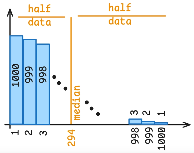
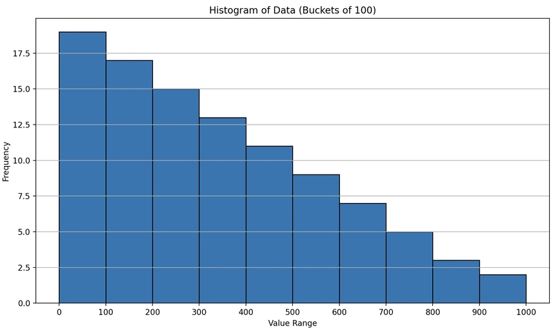
This creates a table with 500,500 rows, where 1 is repeated 1000 times, 2 is repeated 999 times, and so on, until 1000 which is repeated only once. This distribution is shown in the following diagram:
The blog post also demonstrates the concept of histogram bounds in Postgres, which can be observed after analyzing the table:
analyze t;

select
  histogram_bounds::text::int[] as histogram_bounds
from pg_stats
where tablename = 't';
The output is based on a random sampling of the table, so your mileage may vary:
5, 18, 32, 40, 54, 68, 80, 100, 110, 119, 125, 136, 144, 149,
154, 160, 165, 171, 178, 182, 189, 195, 202, 211, 216, 222,
227, 234, 239, 245, 250, 256, 261, 268, 273, 278, 283, 289,
295, 301 307, 314, 320, 325, 332, 339, 346, 352, 358, 364,
370, 376, 383, 389, 396, 402, 409, 415, 422, 429 436, 443,
450, 458, 466, 473, 481, 489, 496, 503, 511, 519, 527, 536,
545, 555, 564, 573, 583, 593 603, 613, 623, 633, 645, 657,
668, 680, 693, 706, 721, 734, 749, 765, 783, 802, 824, 846,
873, 910, 994
The expectation is that the histogram would reflect this skewed distribution, assigning more histogram buckets to regions with higher data density.
Reader Observation: Histogram Does Not Match Intuition
Chris Jones, a reader of the blog, made a sharp observation:
In your out of
histogram_boundsfor table t above, it shows that there are 7 buckets for values 0-100, and 17 buckets for 200-300, even though we know that there are more records with values in the 0-100 range. I got similar bounds when I ran the same example. I tried with lots of different statistics_target values and always got the same. It seems like this histogram implies a distribution that is not correct.
Let's demonstrate his point with actually drawing the bucket distribution for the histogram bounds (using this Python script):
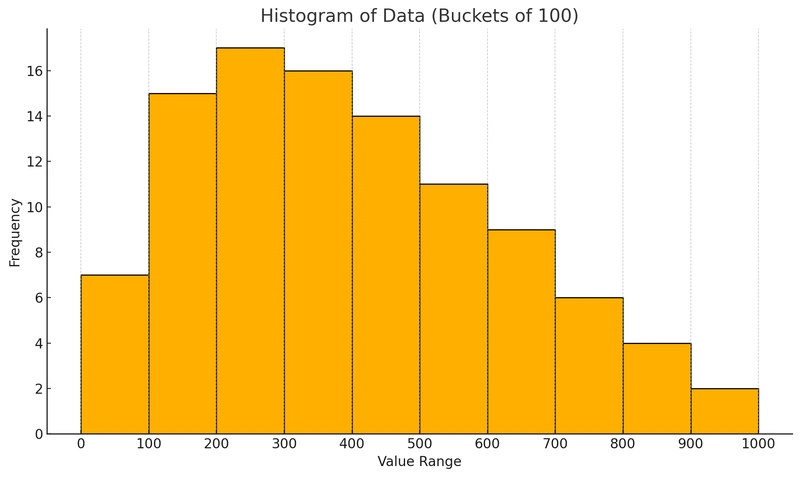
This is an important point. If histogram bounds are used for cardinality estimation, shouldn't denser regions have finer granularity?
Digging Deeper: Why Is the Histogram Counterintuitive?
To understand this, I looked at the PostgreSQL source code. Specifically, this comment in analyze.c explains part of the logic:
/*
 * Generate a histogram slot entry if there are at least two distinct
 * values not accounted for in the MCV list. (This ensures the
 * histogram won't collapse to empty or a singleton.)
 */
This suggests that duplicate values are skipped when building the histogram. To confirm, I checked the implementation further and found that if a value is a duplicate of the previous bound, PostgreSQL will skip it and look for the next distinct value.
In our case, the data contains many duplicate values. These duplicates are not used as histogram boundaries, which causes the histogram to appear flatter than it actually is in the dense region.
Verifying the Hypothesis
To test this explanation, I modified the data by adding a small random offset to each value. This ensures that every value is unique (or nearly unique), avoiding the issue of duplicate elimination during histogram generation.
drop table if exists t;

create table t(n)
  with (autovacuum_enabled = off)
  as select generate_series(1, i) + random() / 1000.0
  from generate_series(1, 1000) as i;

analyze t;

select
  histogram_bounds::text::float[] as histogram_bounds
from pg_stats
where tablename = 't';
With this change, the histogram bounds now behave as expected: the 0–100 range contains many more histogram boundaries than the 100–200 and 200–300 ranges. This better reflects the actual density of the data.
Conclusion
PostgreSQL's histogram statistics do account for data distribution, but the internal logic excludes duplicate values when selecting histogram boundaries. As a result, in datasets with many repeated values, especially in dense regions, the histogram may not appear to reflect the true distribution.
By adding slight randomness to the data, you can force PostgreSQL to treat each value as distinct, which results in more accurate histogram segmentation. This behavior is important to understand when diagnosing query planner decisions or when tuning statistics_target for better performance.
Thanks again to Chris Jones for the sharp observation that triggered a deeper dive into how PostgreSQL builds histograms.