Quantum Information Processing: Foundations - Part 1

For better formatting of math, citations, and all, it is recommended to visit https://johnowolabiidogun.dev/blog/quantum-information-processing-foundations-part-1-9e816e/6801dc9d6e2495ac3e5db09c. Also, part 2 is already posted there. Introduction For decades, computation has mostly been carried out via machines that represent data in one of two states: 000 or 111 . These machines, most probably including the one you are reading this with, are classified as classical computers. The rise in the study of quantum mechanics and information theory in the last decades of the twentieth century birthed a more powerful alternative [@Rieffel2011] termed Quantum Computing (QC), a term commonly attributed to Richard Feynman and the independent work of Yuri Manin [@Rieffel2011]. QC extends classical computing's data representation to include "superposed" (linear combinations) states — which can be infinite [@Bernhardt2019]. This idea of superposition is the cornerstone of this computing paradigm. And instead of classical computers' bitbitbit , quantum computers' base unit is qubitqubitqubit — an abbreviation of quantum and bit, coined by Ben Schumacher in his 1995 "Quantum coding" paper [@Schumacher1995]. In simple terms, QC fundamentally, using Mathematics and Physics, supercharges computing. As demonstrated by Deutsch-Jozsa, Simon, Grover, and Shor's algorithms (which will be discussed in this series), we can have speedups ranging from quadratic to exponential in computational algorithms. Certain encryption protocols have, as reported in October 2024, been broken by Chinese researchers using a quantum algorithm [@Swayne2024]. In this series, we'll be introduced to the theories of QC from notations, measurements, superposition, and entanglement to sophisticated algorithms such as Grover's and Shor's. We will use worked mathematical examples accompanied (mostly) by code verification (using Qiskit and/or Cirq). Most of the problems will be taken from [@Rieffel2011], and their mathematical solutions will be more thoroughly explained for clarity. This is to really understand the concepts. I suggest you check out [@Rieffel2011,@Bernhardt2019] for deeper or more theoretically approachable knowledge. Prerequisite Quantum computing relies on mathematical principles, but you can learn the essentials without being a math whiz. A working knowledge of high school math will equip you to understand the applications and fundamental ideas. Familiarity with the Python programming language will be helpful to understand qiskit and/or cirq code. Dirac notation In quantum mechanics/physics, Dirac notation, named after Paul Adrien Maurice Dirac, the English Mathematician and Theoretical Physicist who developed it in the 1930s, is used to depict quantum states alongside their transformations [@Rieffel2011]. It is composed of two vectors: ∣ψ⟩\ket{\psi}∣ψ⟩ and ⟨ψ∣\bra{\psi}⟨ψ∣ . ∣ψ⟩\ket{\psi}∣ψ⟩ , termed ketketket , represents the column vector of the quantum states whereas ⟨ψ∣\bra{\psi}⟨ψ∣ , regarded as brabrabra , is the row vector. Important things to note here are: ψ†\psi^\daggerψ† is equivalent to the brabrabra , ⟨ψ∣\bra{\psi}⟨ψ∣ , and is obtained by taking the Hermitian (conjugate transpose) of ψ\psiψ . For example, if: ψ=12[1 i]\psi = \frac{1}{\sqrt{2}} \begin{bmatrix} 1 \ i \end{bmatrix} ψ=21[1 i] Then its conjugate transpose (bra) is: ψ†=⟨ψ∣=12[1−i]\psi^\dagger = \bra{\psi} = \frac{1}{\sqrt{2}} \begin{bmatrix} 1 & -i \end{bmatrix} ψ†=⟨ψ∣=21[1−i] This operation involves taking the transpose and then applying complex conjugation to each element [@Lopez2025]. It can then easily be inferred that: ψ⋅ψ†=(12[1 i])⋅(12[1−i]) \psi \cdot \psi^\dagger = \left( \frac{1}{\sqrt{2}} \begin{bmatrix} 1 \ i \end{bmatrix} \right) \cdot \left( \frac{1}{\sqrt{2}} \begin{bmatrix} 1 & -i \end{bmatrix} \right) ψ⋅ψ†=(21[1 i])⋅(21[1−i]) =12[1 i][1−i]=12[1⋅11⋅(−i) i⋅1i⋅(−i)]=12[1−i i1] = \frac{1}{2} \begin{bmatrix} 1 \ i \end{bmatrix} \begin{bmatrix} 1 & -i \end{bmatrix} = \frac{1}{2} \begin{bmatrix} 1 \cdot 1 & 1 \cdot (-i) \ i \cdot 1 & i \cdot (-i) \end{bmatrix} = \frac{1}{2} \begin{bmatrix} 1 & -i \ i & 1 \end{bmatrix} =21[1 i][1−i]=21[1⋅11⋅(−i) i⋅1i⋅(−i)]=21[1−i i1] Note that ψ⋅ψ†≠I\psi \cdot \psi^\dagger \neq Iψ⋅ψ†=I , but instead produces a projection matrix. If we instead compute: ψ†⋅ψ=(12[1−i])⋅(12[1 i]) \psi^\dagger \cdot \psi = \left( \frac{1}{\sqrt{2}} \begin{bmatrix} 1 & -i \end{bmatrix} \right) \cdot \left( \frac{1}{\sqrt{2}} \begin{bmatrix} 1 \ i \end{bmatrix} \right) ψ†⋅ψ=(21[1−i])⋅(21[1 i]) =12(1⋅1+(−i)⋅i)=12(1+1)=1= \frac{1}{2} \left( 1 \cdot 1 + (-i) \cdot i \right) = \frac{1}{2} \left( 1 + 1 \right) = 1 =21(1⋅1+(−i)⋅i)=21(1+1)=1 So we conclude that the inner product (braket) is 111 : ⟨ψ∣ψ⟩=1\braket{\psi|\psi

Apr 23, 2025 - 15:39

Quantum Information Processing: Foundations - Part 1

For better formatting of math, citations, and all, it is recommended to visit https://johnowolabiidogun.dev/blog/quantum-information-processing-foundations-part-1-9e816e/6801dc9d6e2495ac3e5db09c. Also, part 2 is already posted there.

Introduction

For decades, computation has mostly been carried out via machines that represent data in one of two states: $0$ or $1$ . These machines, most probably including the one you are reading this with, are classified as classical computers. The rise in the study of quantum mechanics and information theory in the last decades of the twentieth century birthed a more powerful alternative [@Rieffel2011] termed Quantum Computing (QC), a term commonly attributed to Richard Feynman and the independent work of Yuri Manin [@Rieffel2011]. QC extends classical computing's data representation to include "superposed" (linear combinations) states — which can be infinite [@Bernhardt2019]. This idea of superposition is the cornerstone of this computing paradigm. And instead of classical computers' $bi t$ , quantum computers' base unit is $q u bi t$ — an abbreviation of quantum and bit, coined by Ben Schumacher in his 1995 "Quantum coding" paper [@Schumacher1995]. In simple terms, QC fundamentally, using Mathematics and Physics, supercharges computing. As demonstrated by Deutsch-Jozsa, Simon, Grover, and Shor's algorithms (which will be discussed in this series), we can have speedups ranging from quadratic to exponential in computational algorithms. Certain encryption protocols have, as reported in October 2024, been broken by Chinese researchers using a quantum algorithm [@Swayne2024].

In this series, we'll be introduced to the theories of QC from notations, measurements, superposition, and entanglement to sophisticated algorithms such as Grover's and Shor's. We will use worked mathematical examples accompanied (mostly) by code verification (using Qiskit and/or Cirq). Most of the problems will be taken from [@Rieffel2011], and their mathematical solutions will be more thoroughly explained for clarity. This is to really understand the concepts. I suggest you check out [@Rieffel2011,@Bernhardt2019] for deeper or more theoretically approachable knowledge.

Prerequisite

Quantum computing relies on mathematical principles, but you can learn the essentials without being a math whiz. A working knowledge of high school math will equip you to understand the applications and fundamental ideas. Familiarity with the Python programming language will be helpful to understand qiskit and/or cirq code.

Dirac notation

In quantum mechanics/physics, Dirac notation, named after Paul Adrien Maurice Dirac, the English Mathematician and Theoretical Physicist who developed it in the 1930s, is used to depict quantum states alongside their transformations [@Rieffel2011]. It is composed of two vectors: $∣ψ⟩\ket{\psi}$ and $⟨ψ∣\bra{\psi}$ . $∣ψ⟩\ket{\psi}$ , termed $k e t$ , represents the column vector of the quantum states whereas $⟨ψ∣\bra{\psi}$ , regarded as $b r a$ , is the row vector.

Important things to note here are:

$ψ†\psi^\dagger$ is equivalent to the $b r a$ , $⟨ψ∣\bra{\psi}$ , and is obtained by taking the Hermitian (conjugate transpose) of $ψ\psi$ . For example, if:

i]\psi = \frac{1}{\sqrt{2}} \begin{bmatrix} 1 \ i \end{bmatrix}

Then its conjugate transpose (bra) is:

ψ†=⟨ψ∣=12[1−i]\psi^\dagger = \bra{\psi} = \frac{1}{\sqrt{2}} \begin{bmatrix} 1 & -i \end{bmatrix}

This operation involves taking the transpose and then applying complex conjugation to each element [@Lopez2025]. It can then easily be inferred that:

\psi \cdot \psi^\dagger = \left( \frac{1}{\sqrt{2}} \begin{bmatrix} 1 \ i \end{bmatrix} \right) \cdot \left( \frac{1}{\sqrt{2}} \begin{bmatrix} 1 & -i \end{bmatrix} \right)

\frac{1}{2} \begin{bmatrix} 1 \ i \end{bmatrix} \begin{bmatrix} 1 & -i \end{bmatrix} = \frac{1}{2} \begin{bmatrix} 1 \cdot 1 & 1 \cdot (-i) \ i \cdot 1 & i \cdot (-i) \end{bmatrix} = \frac{1}{2} \begin{bmatrix} 1 & -i \ i & 1 \end{bmatrix}

Note that $ψ⋅ψ†≠I\psi \cdot \psi^\dagger \neq I$ , but instead produces a projection matrix. If we instead compute:

\psi^\dagger \cdot \psi = \left( \frac{1}{\sqrt{2}} \begin{bmatrix} 1 & -i \end{bmatrix} \right) \cdot \left( \frac{1}{\sqrt{2}} \begin{bmatrix} 1 \ i \end{bmatrix} \right)

\frac{1}{2} \left( 1 \cdot 1 + (-i) \cdot i \right) = \frac{1}{2} \left( 1 + 1 \right) = 1

So we conclude that the inner product (braket) is $1$ :

⟨ψ∣ψ⟩=1\braket{\psi|\psi} = 1

However, if $ψ\psi$ is $u ni t a ry$ — a matrix whose inverse is equal to its conjugate transpose — then:

ψ†⋅ψ=ψ⋅ψ†=I\psi^\dagger \cdot \psi = \psi \cdot \psi^\dagger = I

For example, consider the Hadamard gate $H$ :

\frac{1}{\sqrt{2}} \begin{bmatrix} 1 & 1 \ 1 & -1 \end{bmatrix}

Its Hermitian conjugate is:

1−1]H^\dagger = H^T = \frac{1}{\sqrt{2}} \begin{bmatrix} 1 & 1 \ 1 & -1 \end{bmatrix}

Since all entries are real. Then:

H^\dagger H = \frac{1}{2} \begin{bmatrix} 1 & 1 \ 1 & -1 \end{bmatrix} \begin{bmatrix} 1 & 1 \ 1 & -1 \end{bmatrix} = \frac{1}{2} \begin{bmatrix} 1+1 & 1-1 \ 1-1 & 1+1 \end{bmatrix} = \begin{bmatrix} 1 & 0 \ 0 & 1 \end{bmatrix} = I

Therefore, $H$ is unitary. All quantum gates (to be discussed) are unitary.

While the inner product results in a number (scalar), the outer product, $∣ψ⟩⟨ψ∣\ket{\psi}\bra{\psi}$ , produces a matrix:

\ket{\psi}\bra{\psi} = \frac{1}{2} \begin{bmatrix} 1 \ i \end{bmatrix} \begin{bmatrix} 1 & -i \end{bmatrix} = \frac{1}{2} \begin{bmatrix} 1 & -i \ i & 1 \end{bmatrix}

This outer product is a nifty tool for converting matrices to Dirac notation.

In a Hilbert space (quantum vector space), states like $∣0⟩\ket{0}$ and $∣1⟩\ket{1}$ are:
- Orthogonal: $⟨0∣1⟩=0\braket{0|1} = 0$
- Normalized: $⟨0∣0⟩=1\braket{0|0} = 1$

Superposition Principle and Measurements

In quantum mechanics, as in general physics, a system remains in an indeterminate state until it is measured. Quantum states are typically represented in superpositions, following the superposition principle, which states [@Shor2025]:

Let $∣a⟩\ket{a}$ and $∣b⟩\ket{b}$ be two quantum states that are perfectly distinguishable — that is, orthogonal. If $α\alpha$ and $β\beta$ are complex numbers such that the sum of their squared magnitudes is $1$ , then the linear combination (superposition):

α∣a⟩+β∣b⟩\alpha \ket{a} + \beta \ket{b}

is a valid quantum state.

An important takeaway here is the condition that "the sum of their squared magnitudes is 1". This is the simplified consequence of the Born rule, formulated by the German-British physicist Max Born in his 1926 paper [@Born1926].

In QC, measurements are more nuanced, as there are multiple possible measurement bases. The most commonly used is the computational basis, consisting of the states
$∣0⟩\ket{0}$ and $∣1⟩\ket{1}$ . Let's go through examples (Exercise 2.6 in [@Rieffel2011]) of how to measure in QC.

Question 1:

Describe the possible measurement outcome and give the probability for the outcome for this pair consisting of a state and a measurement basis:

\ket{\psi} = \frac{\sqrt{3}}{2}\ket{0} + \frac{1}{2}\ket{1}, {\ket{0}, \ket{1}}

Solution:

When a quantum state is subjected to a measurement in a specific basis, the possible results of that measurement directly correspond to the states that constitute the measurement basis. In this case, since the measurement basis is $∣0⟩,∣1⟩{\ket{0}, \ket{1}}$ , the possible outcomes of measuring the state $∣ψ⟩\ket{\psi}$ are obtaining the state $∣0⟩\ket{0}$ or obtaining the state $∣1⟩\ket{1}$ .

Now, let's proceed to estimate its probabilities:

\mathcal{P}_{\ket{0}} = \left|\frac{\sqrt{3}}{2}\right|^{2} = \frac{3}{4}

\mathcal{P}_{\ket{1}} = \left|\frac{1}{2}\right|^{2} = \frac{1}{4}

Check:

Recall that from the Born rule [@Born1926], a state:

∣ψ⟩=α∣0⟩+β∣1⟩\ket{\psi} = \alpha\ket{0} + \beta\ket{1}

must have its probabilities (squares of the amplitudes) equal to $1$ :

∣α∣2+∣β∣2=1\left|\alpha\right|^{2} + \left|\beta\right|^{2} = 1

\mathcal{P}{\ket{0}} + \mathcal{P}{\ket{1}} = \frac{3}{4} + \frac{1}{4} = \frac{1 + 3}{4} = 1

Code implementation using Google `cirq`

To begin, we need to define a $q u bi t$ in Cirq. This can be done using cirq.NamedQubit or cirq.LineQubit. For this example, we will use cirq.NamedQubit. Next, we create a quantum circuit using cirq.Circuit(). To prepare the desired quantum state $∣ψ⟩=32∣0⟩+12∣1⟩\ket{\psi} = \frac{\sqrt{3}}{2}\ket{0} + \frac{1}{2}\ket{1}$ , we will define the target state vector with numpy.array and pass its result in cirq.StatePreparationChannel.

There is another, more mathematical and accurate way to do this, using rotation, but since we haven't introduced the concept yet, we will go with this.

Then, to verify the probabilities, we need to add a measurement operation to the circuit in the computational basis. Cirq provides the cirq.measure() function or the cirq.MeasurementGate for this purpose. To retrieve the results, we need to simulate the quantum circuit. cirq.Simulator() shines here. The complete code is now:

import cirq
import numpy as np

# Define a qubit
q = cirq.NamedQubit('q')

# Create a circuit
circuit = cirq.Circuit()

# Define the target state vector
target_state = np.array([np.sqrt(3)/2, 1/2])

# Prepare the state using StatePreparationChannel
circuit.append(cirq.StatePreparationChannel(target_state).on(q))

# Add a measurement operation
circuit.append(cirq.measure(q, key='result'))

print("Circuit to prepare the state:")
print(circuit)

# Create a simulator
simulator = cirq.Simulator()

# Run the simulation multiple times
repetitions = 1000
result = simulator.run(circuit, repetitions=repetitions)

# Get the measurement results
measurement_counts = result.histogram(key='result')
print(f"\nMeasurement counts after {repetitions} repetitions:")
print(measurement_counts)

# Calculate the probabilities from the simulation
probability_0 = measurement_counts.get(0, 0) / repetitions
probability_1 = measurement_counts.get(1, 0) / repetitions

print(f"\nSimulated probability of outcome 0: {probability_0:.3f}")
print(f"Simulated probability of outcome 1: {probability_1:.3f}")

Question 2:

Describe the possible measurement outcome and give the probability for the outcome for this pair consisting of a state and a measurement basis:

∣ψ⟩=∣−i⟩,∣0⟩,∣1⟩\ket{\psi} = \ket{-i}, {\ket{0}, \ket{1}}

Solution

The measurement basis for this is exactly equal to the previous one. It's only the state that differs. So the possible outcomes still hold.

Let's zoom in on the state:

∣ψ⟩=∣−i⟩\ket{\psi} = \ket{-i}

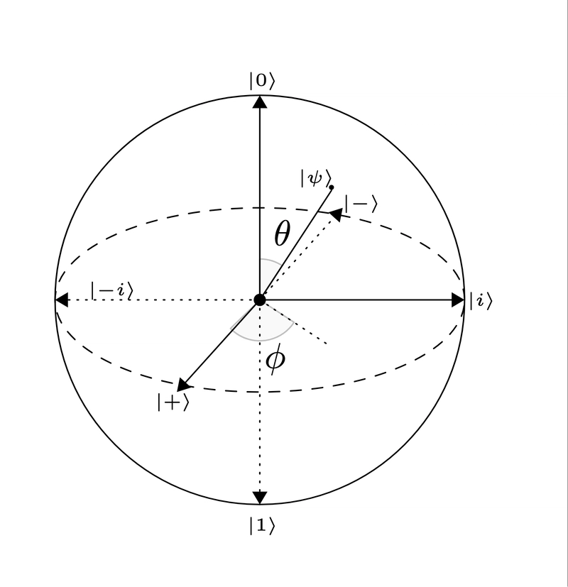
We'll introduce the concept of the Bloch Sphere here.

The Bloch Sphere is a geometric representation of a qubit's state space, which helps visualize superposition.

Here's an illustration:

{Figure 1: Bloch Sphere showing the major measurement basis.}

According to the Bloch Sphere (will be discussed more later) above, the given state:

∣−i⟩=12(∣0⟩−i∣1⟩)=12∣0⟩−12i∣1⟩\ket{-i} = \frac{1}{\sqrt{2}}\left( \ket{0} - i\ket{1} \right) = \frac{1}{\sqrt{2}}\ket{0} -\frac{1}{\sqrt{2}}i\ket{1}

From this, their probabilities are calculated as follows:

\mathcal{P}_{\ket{0}} = \left| \frac{1}{\sqrt{2}} \right|^{2} = \frac{1}{2}

\mathcal{P}_{\ket{1}} = \left| -\frac{1}{\sqrt{2}}i \right|^{2} = \left| - i \right|^{2} \times \left| \frac{1}{\sqrt{2}} \right|^{2} = - \times -1 \times \frac{1}{2} = \frac{1}{2}

Since $i2=(−1)2=−1i^2 = (\sqrt{-1})^2= -1$ .

Check:

$P∣0⟩+P∣1⟩=12+12=1\mathcal{P}{\ket{0}} + \mathcal{P}{\ket{1}} = \frac{1}{2} + \frac{1}{2} = 1$ .

Simulating the circuit with Qiskit or Cirq is left as an exercise to the reader.

Question 3:

Describe the possible measurement outcome and give the probability for the outcome for this pair consisting of a state and a measurement basis:

∣ψ⟩=∣0⟩,∣+⟩,∣−⟩\ket{\psi} = \ket{0}, {\ket{+}, \ket{-}}

Solution

As mentioned earlier, when a quantum system is measured with respect to a particular basis, the possible outcomes of that measurement are the basis states themselves. In this scenario, the measurement is performed in the Hadamard basis, which is comprised of the states $∣+⟩\ket{+}$ and $∣−⟩\ket{-}$ . Consequently, the only possible outcomes of measuring a qubit in the ${+}, \ket{-}}$ basis are the qubit collapsing into either the $∣+⟩\ket{+}$ state or the $∣−⟩\ket{-}$ state.

To find the probabilities of these outcomes, we need to know that:

∣+⟩≡∣0⟩+∣1⟩2\ket{+} \equiv \frac{\ket{0} + \ket{1}}{\sqrt{2}}

∣−⟩≡∣0⟩−∣1⟩2\ket{-} \equiv \frac{\ket{0} - \ket{1}}{\sqrt{2}}

and that the given state, $∣0⟩\ket{0}$ , is:

∣0⟩=12(∣+⟩+∣−⟩)\ket{0} = \frac{1}{\sqrt{2}}\left(\ket{+} + \ket{-} \right)

From here, we can simply estimate the probabilities of each of the outcomes:

\mathcal{P}_{\ket{+}} = \left| \frac{1}{\sqrt{2}} \right|^{2} = \frac{1}{2}

\mathcal{P}_{\ket{-}} = \left| \frac{1}{\sqrt{2}} \right|^{2} = \frac{1}{2}

Another approach (which works for even the preceding and succeeding exercises since it's fundamental) is to use the idea of inner product. Since the measurement basis is ${+}, \ket{-}}$ and the given state is $∣0⟩\ket{0}$ , the probability of each measurement outcome is the square of the inner product of the state with the measurement outcome. In other words:

P∣+⟩=∣⟨+∣0⟩∣2\mathcal{P}{\ket{+}} = \left|\braket{+|0}\right|^2

P∣−⟩=∣⟨−∣0⟩∣2\mathcal{P}{\ket{-}} = \left|\braket{-|0}\right|^2

$∴\therefore$

\mathcal{P}_{\ket{+}} = \left| \braket{\frac{1}{\sqrt{2}}(\ket{0} + \ket{1})|0} \right|^2 = \frac{1}{2}\left| (\bra{0} + \bra{1})\ket{0} \right|^2

The $b r a$ simply transforms $∣0⟩\ket{0}$ and $∣1⟩\ket{1}$ to row vectors: $⟨0∣\bra{0}$ and $⟨1∣\bra{1}$ . Multiplying out:

\mathcal{P}_{\ket{+}} = \frac{1}{2}\left| \braket{0|0} + \braket{1|0} \right|^2 = \frac{1}{2}|1+0|^2 = \frac{1}{2}

Similarly,

\mathcal{P}_{\ket{-}} = \left| \braket{\frac{1}{\sqrt{2}}(\ket{0} - \ket{1})|0} \right|^2 = \frac{1}{2}\left| (\bra{0} - \bra{1})\ket{0} \right|^2

\frac{1}{2}\left| \braket{0|0} - \braket{1|0} \right|^2 = \frac{1}{2}|1-0|^2 = \frac{1}{2}

Check

This is another cirq code for this:

import cirq
import numpy as np

# Define a qubit
qubit = cirq.LineQubit(0)

# Create a quantum circuit
circuit = cirq.Circuit()

# The qubit is initialized to |0>

# Apply a Hadamard gate to prepare for measurement in the Hadamard basis
circuit.append(cirq.H(qubit))

# Measure the qubit in the computational basis
circuit.append(cirq.measure(qubit, key='result'))

# Print the circuit
print("Quantum Circuit:")
print(circuit)

# Simulate the circuit many times to get probabilities
simulator = cirq.Simulator()
num_simulations = 1000
results = simulator.run(circuit, repetitions=num_simulations)

# Get the measurement results
measurement_outcomes = results.measurements['result']

# Count the occurrences of each outcome (0 and 1)
counts = np.unique(measurement_outcomes, return_counts=True)
print(f'{counts[0][0]}: {counts[1][0]}')
print(f'{counts[0][1]}: {counts[1][1]}')

# Calculate the probabilities of each outcome
probability_0 = counts[1][0] / num_simulations
probability_1 = counts[1][1] / num_simulations

print("\nSimulation Results:")
print(f"Number of simulations: {num_simulations}")
print(f"Probability of outcome 0 (corresponding to |+>): {probability_0:.3f}")
print(f"Probability of outcome 1 (corresponding to |->): {probability_1:.3f}")

Question 4:

Describe the possible measurement outcome and give the probability for the outcome for this pair consisting of a state and a measurement basis:

\ket{\psi} = \frac{1}{\sqrt{2}}\left( \ket{0} - \ket{1} \right), {\ket{i}, \ket{-i}}

Solution

Again, since the state is measured in $∣i⟩,∣−i⟩{\ket{i}, \ket{-i}}$ , the possible measurement outcomes are obtaining the system in the state $∣i⟩\ket{i}$ or in the state $∣−i⟩\ket{-i}$ .

Now, there are two approaches to finding the probabilities of these outcomes. We will explore the fundamental (inner product) approach first.

Recall that:

Given a state $∣ψ⟩\ket{\psi}$ , the probability of each of the measurement outcomes in the given basis is the square of the inner product of the state with each of the measurement outcomes.

and (from the Bloch Sphere):

\begin{gather} \ket{i} = \frac{1}{\sqrt{2}}(\ket{0} + i\ket{1}) \ \bra{i} = \frac{1}{\sqrt{2}}(\bra{0} - i\bra{1}) \end{gather}

\begin{gather} \ket{-i} = \frac{1}{\sqrt{2}}(\ket{0} - i\ket{1}) \ \bra{-i} = \frac{1}{\sqrt{2}}(\bra{0} + i\bra{1}) \end{gather}

Therefore,

P∣i⟩=∣⟨i∣ψ⟩∣2\mathcal{P}{\ket{i}} = |\braket{i|\psi}|^2

P∣−i⟩=∣⟨−i∣ψ⟩∣2\mathcal{P}{\ket{-i}} = |\braket{-i|\psi}|^2

Let's expand $P∣i⟩\mathcal{P}_{\ket{i}}$ out first:

ParseError: KaTeX parse error: Expected '}', got '\right' at position 138: …{0} + i\ket{1})\̲r̲i̲g̲h̲t̲}|\left{\frac{1…

Given a complex number $z = a + bi$ , its magnitude $\sqrt{a^2 + b^2}$ . So, $\sqrt{1^2 + 1^2} = \sqrt{2}$ .

$∴\therefore$

\mathcal{P}_{\ket{i}}= \frac{1}{4}(\sqrt{2})^2 = \frac{1}{4}\cdot2 = \frac{1}{2}

In the same vein, $P∣−i⟩\mathcal{P}_{\ket{-i}}$ is estimated as follows:

ParseError: KaTeX parse error: Expected '}', got '\right' at position 140: …{0} - i\ket{1})\̲r̲i̲g̲h̲t̲}|\left{\frac{1…

Of course, they obey the Born rule.

A second approach is to flex some mathematical muscle and some intuition derived from the fact that the given state can be expressed in terms of the measurement basis.

Imagine $α\alpha$ and $β\beta$ coefficients such that:

\begin{equation} \tag{3i} \ket{\psi} = a\ket{i} + b\ket{-i} \end{equation}

Substituting $(1)$ and $(3)$ into $(3 i)$ :

\begin{align} \notag \frac{1}{\sqrt{2}}\left( \ket{0} - \ket{1} \right) &= \alpha \cdot \frac{1}{\sqrt{2}}\left( \ket{0} + i\ket{1} \right) + \beta \cdot \frac{1}{\sqrt{2}}\left( \ket{0} - i\ket{1} \right)\ \frac{1}{\sqrt{2}}\ket{0} + \frac{-1}{\sqrt{2}}\ket{1} &= \frac{\alpha + \beta}{\sqrt{2}}\ket{0} + \frac{\alpha i - \beta i}{\sqrt{2}}\ket{1} \end{align}

Comparing both sides of $(5)$ with the respective values of $∣0⟩\ket{0}$ and $∣1⟩\ket{1}$ :

\begin{align} \notag \frac{1}{\sqrt{2}}\ket{0} &= \frac{\alpha + \beta}{\sqrt{2}}\ket{0}\ \tag{3ii} \alpha + \beta &= 1 \end{align}

and

\begin{align} \notag \frac{-1}{\sqrt{2}}\ket{1} &= \frac{\alpha i - \beta i}{\sqrt{2}}\ket{1}\ \notag \alpha i - \beta i &= -1\ \notag i (\alpha - \beta) &= - 1\ \notag \alpha - \beta &= \frac{-1}{i} = \frac{-1}{i}\cdot\frac{i}{i} = \frac{-i}{i^2} = \frac{-i}{-1} \ \tag{3iii} \alpha - \beta &= i \end{align}

Solve $(3 ii)$ and $(3 iii)$ simultaneously by adding them together (substitution method),

ParseError: KaTeX parse error: Too many tab characters: & at position 77: …\alpha - \beta &̲= i \end{split}…

\begin{align} \notag 2\alpha &= 1 + i\ \tag{3iv} \alpha &= \frac{1+i}{2} \end{align}

Let's substitute $α\alpha$ in $(3 ii)$ :

\begin{align} \notag \frac{1+i}{2} + \beta &= 1\ \notag \beta &= 1 - \frac{1+i}{2}\ \tag{3v} \beta &= \frac{2 - (1+i)}{2} = \frac{1-i}{2} \end{align}

With these, our imagined expression becomes:

\ket{\psi} = \frac{1 + i}{2}\ket{i} + \frac{1 - i}{2} \ket{-i}

So,

\mathcal{P}_{\ket{i}} = \left|\frac{1}{2} (1 + i)\right|^{2} = \left|\frac{1}{2}\right|^{2} \times |(1 + i)|^2 = \frac{1}{4} \times \left(\sqrt{1^2 + (1)^2}\right)^2 = \frac{1}{4} \times 2 = \frac{1}{2}

\mathcal{P}_{\ket{-i}} = \left|\frac{1}{2} (1 - i)\right|^{2} = \left|\frac{1}{2}\right|^{2} \times |(1 - i)|^2 = \frac{1}{4} \times \left(\sqrt{1^2 + (-1)^2}\right)^2 = \frac{1}{4} \times 2 = \frac{1}{2}

Arriving at the same answers with the first approach, though longer.

Any of these approaches can be used to tackle problems of this nature. The first approach is quite a generalist!

Before closing up here, let's write a cirq simulation for this:

import cirq
import numpy as np

qubit = cirq.LineQubit(0)
psi_preparation = cirq.Circuit(cirq.H(qubit), cirq.Z(qubit))
print("Circuit for preparing psi:")
print(psi_preparation)

# This is based on some unitary transformations since, by default, `cirq.measure`
# perform standard measurements in the computational basis (Z-basis)
# and to measure in another basis, we need to do the unitary transformations that map
# this |i>, |-i> to the computational basis before performing the measurement
measurement_basis_transformation = cirq.Circuit(cirq.S(qubit)**-1, cirq.H(qubit))
measurement_circuit = psi_preparation + measurement_basis_transformation + cirq.Circuit(cirq.measure(qubit, key='result'))
print("\nCircuit for measurement in the {|i>, |-i>} basis:")
print(measurement_circuit)

simulator = cirq.Simulator()
num_repetitions = 1000
results = simulator.run(measurement_circuit, repetitions=num_repetitions)
measurement_counts = results.histogram(key='result')
print("\nMeasurement counts:", measurement_counts)

probability_i = measurement_counts.get(0, 0) / num_repetitions
probability_minus_i = measurement_counts.get(1, 0) / num_repetitions
print(f"Probability of outcome corresponding to |i>: {probability_i:.3f}")
print(f"Probability of outcome corresponding to |-i>: {probability_minus_i:.3f}")

Outro

Enjoyed this article? I'm a Software Engineer and Technical Writer actively seeking new opportunities to impact and learn, particularly in areas related to web security, finance, healthcare, and education. If you think my expertise aligns with your team's needs, let's chat! You can find me on LinkedIn and X. I am also an email away.

References
[@Rieffel2011]: Rieffel, E. G., & Polak, W. H. (2014). Quantum Computing: A Gentle Introduction. MIT Press. https://books.google.com/books?id=CQ3YoAEACAAJ
[@Bernhardt2019]: Bernhardt, C. (2019). Quantum Computing for Everyone. The MIT Press.
[@Schumacher1995]: Schumacher, B. (1995). Quantum coding. Physical Review A, 51(4), 2738-2747.
[@Swayne2024]: Swayne, M. (2024). Chinese scientists report using quantum computer to hack military-grade encryption. The Quantum Insider. https://thequantuminsider.com/2024/10/11/chinese-scientists-report-using-quantum-computer-to-hack-military-grade-encryption/. Retrieved April 17, 2025
[@Lopez2025]: Lopez, S., Hudek, T., Li, M., Hansen, D. P., Sánchez, E. G. & Gronlund, C. J. (2025). Dirac notation in quantum computing. Microsoft Learn. https://learn.microsoft.com/en-us/azure/quantum/concepts-dirac-notation. Retrieved April 17, 2025
[@Shor2025]: Shor, P. (2022). Lecture 2: Quantum Computation. MIT Mathematics. https://math.mit.edu/~shor/435-LN/Lecture_02.pdf. Retrieved April 17, 2025
[@Born1926]: Born, M. (1926). Zur Quantenmechanik der Stoßvorgänge. Zeitschrift für Physik, 37(12), 863-867.