InsightFlow Part 5: Designing the Data Model & Schema with dbt for InsightFlow

InsightFlow GitHub Repo In this post, we’ll dive into how the data model and schema for the InsightFlow project were designed using dbt (Data Build Tool). This layer is critical for transforming raw data into a structured, analysis-ready format that supports efficient querying and visualization. We’ll also explore the Entity-Relationship Diagram (ERD) for the project, which provides a visual representation of the relationships between the key entities in the data model. Why dbt for Data Modeling? dbt is a powerful tool for transforming raw data into a structured format using SQL. It enables data engineers to: Standardize Transformations: Define reusable SQL models for data cleaning, normalization, and enrichment. Version Control: Manage transformations as code in Git for collaboration and reproducibility. Test Data Quality: Add tests to ensure data integrity at every stage of the pipeline. Optimize for Querying: Materialize models as views or tables, partitioned and optimized for querying in AWS Athena. For InsightFlow, dbt was the ideal choice to transform raw retail and fuel price data into a star schema that supports analysis of trends and correlations. Overview of the Data Model The InsightFlow data model is designed as a star schema, with the following key components: Fact Table: Contains quantitative metrics, such as sales values and fuel prices. Dimension Tables: Provide descriptive attributes, such as MSIC group codes and dates, to slice and dice the data. Key Tables Fact Table: fct_retail_sales_monthly Metrics: Sales values, volume indices, fuel prices. Partitioned by: Year and month for efficient querying in Athena. Dimension Tables: dim_msic_lookup: Provides descriptions for MSIC group codes. dim_date: A date dimension table for time-based analysis. Step 1: Defining Sources The raw data ingested into the landing zone (S3 bucket) is defined as sources in dbt. These sources are created by the Glue Crawler and include: iowrt: Headline wholesale and retail trade data. iowrt_3d: Detailed wholesale and retail trade data by MSIC group. fuelprice: Weekly fuel price data. Here’s how the sources are defined in sources.yml: version: 2 sources: - name: landing_zone schema: insightflow_prod description: "Raw data loaded from data.gov.my sources via AWS Batch ingestion." tables: - name: iowrt description: "Raw Headline Wholesale & Retail Trade data (monthly)." columns: - name: series description: "Series type ('abs', 'growth_yoy', 'growth_mom')" - name: ymd_date description: "Date of record (YYYY-MM-DD, monthly frequency)" - name: sales description: "Sales Value (RM mil)" - name: volume description: "Volume Index (base 2015 = 100)" - name: fuelprice description: "Raw weekly fuel price data." columns: - name: ron95 description: "RON95 Price (RM/litre)" - name: ron97 description: "RON97 Price (RM/litre)" - name: diesel description: "Diesel Price (RM/litre)" Step 2: Creating Staging Models Staging models clean and standardize the raw data. For example, the stg_iowrt.sql model filters for absolute values and casts columns to appropriate data types: with source_data as ( select series, cast(ymd_date as date) as record_date, sales, volume from {{ source('landing_zone', 'iowrt') }} where series = 'abs' ) select record_date, cast(sales as double) as sales_value_rm_mil, cast(volume as double) as volume_index from source_data Step 3: Building the Fact Table The fact table, fct_retail_sales_monthly, combines data from multiple sources (e.g., retail sales and fuel prices) into a single table. It is partitioned by year and month for efficient querying in Athena. Here’s the configuration in dbt_project.yml: fct_retail_sales_monthly: +materialized: table +partitions: - year - month Step 4: Adding Dimension Tables 1. MSIC Lookup Dimension The dim_msic_lookup table provides descriptions for MSIC group codes. It is created from a seed file (msic_lookup.csv): seeds: insightflow: msic_lookup: +schema: raw_seeds +file_format: parquet +column_types: group_code: varchar desc_en: varchar desc_bm: varchar 2. Date Dimension The dim_date table is a standard date dimension table that supports time-based analysis. Step 5: Testing and Documentation dbt allows you to add tests to ensure data quality. For example, you can test that the sales column in the fact table is not null: tests: - not_null - accepted_values: values: [abs, growth_yoy, growth_mom] Additionally, dbt automatically

Apr 29, 2025 - 04:11

InsightFlow Part 5: Designing the Data Model & Schema with dbt for InsightFlow

In this post, we’ll dive into how the data model and schema for the InsightFlow project were designed using dbt (Data Build Tool). This layer is critical for transforming raw data into a structured, analysis-ready format that supports efficient querying and visualization. We’ll also explore the Entity-Relationship Diagram (ERD) for the project, which provides a visual representation of the relationships between the key entities in the data model.

Why dbt for Data Modeling?

dbt is a powerful tool for transforming raw data into a structured format using SQL. It enables data engineers to:

Standardize Transformations: Define reusable SQL models for data cleaning, normalization, and enrichment.
Version Control: Manage transformations as code in Git for collaboration and reproducibility.
Test Data Quality: Add tests to ensure data integrity at every stage of the pipeline.
Optimize for Querying: Materialize models as views or tables, partitioned and optimized for querying in AWS Athena.

For InsightFlow, dbt was the ideal choice to transform raw retail and fuel price data into a star schema that supports analysis of trends and correlations.

Overview of the Data Model

The InsightFlow data model is designed as a star schema, with the following key components:

Fact Table: Contains quantitative metrics, such as sales values and fuel prices.
Dimension Tables: Provide descriptive attributes, such as MSIC group codes and dates, to slice and dice the data.

Key Tables

Fact Table: fct_retail_sales_monthly
- Metrics: Sales values, volume indices, fuel prices.
- Partitioned by: Year and month for efficient querying in Athena.
Dimension Tables:
- dim_msic_lookup: Provides descriptions for MSIC group codes.
- dim_date: A date dimension table for time-based analysis.

Step 1: Defining Sources

The raw data ingested into the landing zone (S3 bucket) is defined as sources in dbt. These sources are created by the Glue Crawler and include:

iowrt: Headline wholesale and retail trade data.
iowrt_3d: Detailed wholesale and retail trade data by MSIC group.
fuelprice: Weekly fuel price data.

Here’s how the sources are defined in sources.yml:

version: 2

sources:
  - name: landing_zone
    schema: insightflow_prod
    description: "Raw data loaded from data.gov.my sources via AWS Batch ingestion."
    tables:
      - name: iowrt
        description: "Raw Headline Wholesale & Retail Trade data (monthly)."
        columns:
          - name: series
            description: "Series type ('abs', 'growth_yoy', 'growth_mom')"
          - name: ymd_date
            description: "Date of record (YYYY-MM-DD, monthly frequency)"
          - name: sales
            description: "Sales Value (RM mil)"
          - name: volume
            description: "Volume Index (base 2015 = 100)"
      - name: fuelprice
        description: "Raw weekly fuel price data."
        columns:
          - name: ron95
            description: "RON95 Price (RM/litre)"
          - name: ron97
            description: "RON97 Price (RM/litre)"
          - name: diesel
            description: "Diesel Price (RM/litre)"

Step 2: Creating Staging Models

Staging models clean and standardize the raw data. For example, the stg_iowrt.sql model filters for absolute values and casts columns to appropriate data types:

with source_data as (
    select
        series,
        cast(ymd_date as date) as record_date,
        sales,
        volume
    from {{ source('landing_zone', 'iowrt') }}
    where series = 'abs'
)

select
    record_date,
    cast(sales as double) as sales_value_rm_mil,
    cast(volume as double) as volume_index
from source_data

Step 3: Building the Fact Table

The fact table, fct_retail_sales_monthly, combines data from multiple sources (e.g., retail sales and fuel prices) into a single table. It is partitioned by year and month for efficient querying in Athena.

Here’s the configuration in dbt_project.yml:

fct_retail_sales_monthly:
  +materialized: table
  +partitions:
    - year
    - month

Step 4: Adding Dimension Tables

1. MSIC Lookup Dimension

The dim_msic_lookup table provides descriptions for MSIC group codes. It is created from a seed file (msic_lookup.csv):

seeds:
  insightflow:
    msic_lookup:
      +schema: raw_seeds
      +file_format: parquet
      +column_types:
        group_code: varchar
        desc_en: varchar
        desc_bm: varchar

2. Date Dimension

The dim_date table is a standard date dimension table that supports time-based analysis.

Step 5: Testing and Documentation

dbt allows you to add tests to ensure data quality. For example, you can test that the sales column in the fact table is not null:

tests:
  - not_null
  - accepted_values:
      values: [abs, growth_yoy, growth_mom]

Additionally, dbt automatically generates documentation for your models, which can be viewed in a browser.

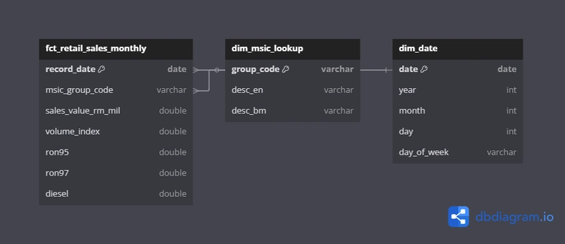
Entity-Relationship Diagram (ERD)

Here’s the ERD for the InsightFlow data model:

You can copy this diagram into dbdiagram.io to visualize the relationships.

Conclusion

By leveraging dbt, we transformed raw data into a structured, analysis-ready format. The star schema design ensures efficient querying and supports a wide range of analyses, from sales trends to fuel price correlations.