Cat or Dog? — Building a Binary Image Classifier with TensorFlow

This article is co-authored by @eerrynnee. Interactive version of the article on Google Colab “Is this a cat or a dog?” A simple question — unless you're asking a computer. A few years ago, the idea of teaching a machine to recognize objects in photos might’ve sounded too far-fetched. These days, it’s something you can do in an afternoon, right from your browser. This article walks you through how to build a basic binary image classifier, one that can tell whether an image contains a cat or a dog. No deep dives into theory, no expensive hardware required. Just some Python, a cloud notebook, and a dataset full of furry creatures. We’ll start by understanding how image data is represented, then build a model using TensorFlow and Keras, and finally train it on real-world images. Along the way, we’ll also reflect on what it means to teach machines to “see”. What is image classification? Image classification is a type of supervised learning where the model learns to associate an input image with a specific category. Binary classification divides unknown data points into two groups and labels images using an either-or logic. In our case: cats and dogs. The model's output is either: 0 for cat 1 for dog What is TensorFlow? TensorFlow is an open-source platform developed by Google for machine learning and deep learning applications. It serves as both a symbolic math library and a robust framework for building complex machine learning models. TensorFlow offers excellent graph representation, supports a variety of backends including GUI and ASIC, and is known for its high performance and strong community support. It also allows easy debugging of graph components and is highly extensible for custom model development. On the other hand, Keras is a high-level neural network library that runs on top of TensorFlow and provides a user-friendly API for building deep learning models. Designed for simplicity and speed, Keras is ideal for beginners and researchers alike. It offers support for multiple backends, includes a collection of pre-trained models, and enjoys strong community support, making it a go-to tool for rapid prototyping and implementation of neural networks. Images as Data When we look at a photo, we instantly see a scene: maybe a cat curled on a rug or a golden retriever wagging its tail. But for a computer, an image is a grid of numbers, and not a visual moment. Every image is made up of pixels, and each pixel holds numerical values that describe its color. These values are typically represented using three color channels: Red, Green, and Blue (RGB). You can think of each channel as a grayscale image that highlights one component of color. So when you load an image into your program, it's actually being read as a 3-dimensional array: Height - the number of vertical pixels Width - the number of horizontal pixels Channels - usually 3 for RGB (sometimes 1 for grayscale, or 4 for RGBA if there's transparency) For example, a 200x200 image with 3 channels would be stored as a 200×200×3 matrix — and every number inside it ranges from 0 to 255, representing intensity (0 = no light, 255 = full light). Obtaining the Data In supervised machine learning, particularly in image classification tasks, the performance of a model is heavily influenced by the quality and size of the dataset it is trained on. For this project, the model is trained on a publicly available dataset containing images of cats and dogs obtained from Kaggle. What is Kaggle? Kaggle is a platform for data science and machine learning specialists where they may compete to build the best models for solving specific issues or analyzing specific data. The site also allows users to collaborate on projects, share code and data sets, and learn from one another's work. We use a dataset titled "dogs vs cats" from Kaggle, uploaded by the user "salader". It consists of colored JPEG images of cats and dogs, each labeled according to its category. The visual diversity within the dataset such as different breeds, postures, and lighting conditions, makes it a valuable resource for training image classification models. In total, the dataset contains around 12500 images per class. This balanced composition is ideal for binary classification tasks, as it helps prevent model bias toward a particular class. Both classes are sorted into their respective test and training directories, which simplifies the preprocessing process. Why Use Google Colab? To efficiently work with this dataset and build models, we will use a tool called Google Colab. Google Colab is a cloud-based Jupyter notebook environment that runs entirely in your browser. It’s ideal for personal machine learning projects because: No setup is required Free access to GPUs Easy integration with Google Drive Supports real-time collaboration Kaggle API setup To utilize the dataset we need from Kaggle, we n

Apr 24, 2025 - 15:07

Cat or Dog? — Building a Binary Image Classifier with TensorFlow

This article is co-authored by @eerrynnee.

Interactive version of the article on Google Colab

“Is this a cat or a dog?”

A simple question — unless you're asking a computer.

A few years ago, the idea of teaching a machine to recognize objects in photos might’ve sounded too far-fetched. These days, it’s something you can do in an afternoon, right from your browser.

This article walks you through how to build a basic binary image classifier, one that can tell whether an image contains a cat or a dog. No deep dives into theory, no expensive hardware required. Just some Python, a cloud notebook, and a dataset full of furry creatures.

We’ll start by understanding how image data is represented, then build a model using TensorFlow and Keras, and finally train it on real-world images. Along the way, we’ll also reflect on what it means to teach machines to “see”.

What is image classification?

Image classification is a type of supervised learning where the model learns to associate an input image with a specific category.

Binary classification divides unknown data points into two groups and labels images using an either-or logic. In our case: cats and dogs. The model's output is either:

0 for cat
1 for dog

What is TensorFlow?

TensorFlow is an open-source platform developed by Google for machine learning and deep learning applications. It serves as both a symbolic math library and a robust framework for building complex machine learning models.

TensorFlow offers excellent graph representation, supports a variety of backends including GUI and ASIC, and is known for its high performance and strong community support. It also allows easy debugging of graph components and is highly extensible for custom model development.

On the other hand, Keras is a high-level neural network library that runs on top of TensorFlow and provides a user-friendly API for
building deep learning models.

Designed for simplicity and speed, Keras is ideal for beginners and researchers alike. It offers support for multiple backends, includes a collection of pre-trained models, and enjoys strong community support, making it a go-to tool for rapid prototyping and implementation of neural networks.

Images as Data

When we look at a photo, we instantly see a scene: maybe a cat curled on a rug or a golden retriever wagging its tail. But for a computer, an image is a grid of numbers, and not a visual moment.

Every image is made up of pixels, and each pixel holds numerical values that describe its color. These values are typically represented using three color channels: Red, Green, and Blue (RGB). You can think of each channel as a grayscale image that highlights one component of color.

So when you load an image into your program, it's actually being read as a 3-dimensional array:

Height - the number of vertical pixels
Width - the number of horizontal pixels
Channels - usually 3 for RGB (sometimes 1 for grayscale, or 4 for RGBA if there's transparency)

For example, a 200x200 image with 3 channels would be stored as a 200×200×3 matrix — and every number inside it ranges from 0 to 255, representing intensity (0 = no light, 255 = full light).

Obtaining the Data

In supervised machine learning, particularly in image classification tasks, the performance of a model is heavily influenced by the quality and size of the dataset it is trained on. For this project, the model is trained on a publicly available dataset containing images of cats and dogs obtained from Kaggle.

What is Kaggle?

Kaggle is a platform for data science and machine learning specialists where they may compete to build the best models for solving specific issues or analyzing specific data. The site also allows users to collaborate on projects, share code and data sets, and learn from one another's work.

We use a dataset titled "dogs vs cats" from Kaggle, uploaded by the user "salader".

It consists of colored JPEG images of cats and dogs, each labeled according to its category. The visual diversity within the dataset such as different breeds, postures, and lighting conditions, makes it a valuable resource for training image classification models.

In total, the dataset contains around 12500 images per class. This balanced composition is ideal for binary classification tasks, as it helps prevent model bias toward a particular class. Both classes are sorted into their respective test and training directories, which simplifies the preprocessing process.

Why Use Google Colab?

To efficiently work with this dataset and build models, we will use a tool called Google Colab.

Google Colab is a cloud-based Jupyter notebook environment that runs entirely in your browser.

It’s ideal for personal machine learning projects because:

No setup is required
Free access to GPUs
Easy integration with Google Drive
Supports real-time collaboration

Kaggle API setup

To utilize the dataset we need from Kaggle, we need to get an API token from kaggle.com.

To get an API token, you need to first register for a free Kaggle account here.

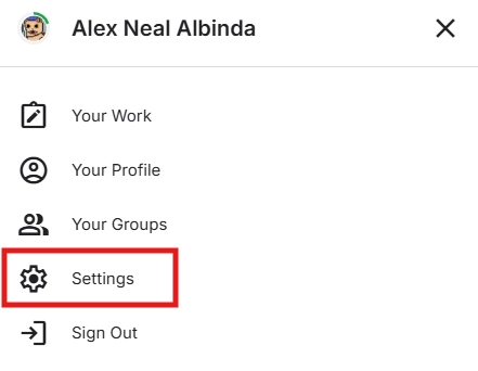
Once you have a Kaggle account, navigate to the settings of your account, and scroll down.

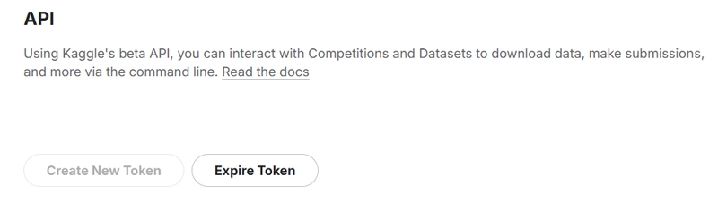
Click on Create New Token, and it should download the kaggle.json file.

If we open kaggle.json on a text editor, for example, Visual Studio Code, we would find two key-value pairs:

{"username":"reallycooluser","key":"12345678909876345678"}

We can input these two values,

KAGGLE_KEY = 12345678909876345678
KAGGLE_USERNAME = reallycooluser

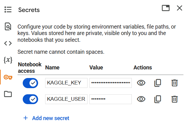
into Google Colab's built in Secrets feature that lets us store our sensitive info, like our Kaggle API key, privately.

Even if the notebook resets, we can still use the same Kaggle token without having to reupload it.

The Secrets feature of Google Colab is found on the left sidebar, with a key icon.

To access the Kaggle API using the Secrets feature, we run the following code block:

# Imports the Kaggle.com key and username from the Google Colab Secrets
from google.colab import userdata
import os

# assuming you followed the naming convention from above:
# KAGGLE_KEY = key
# KAGGLE_USERNAME = username
os.environ["KAGGLE_KEY"] = userdata.get('KAGGLE_KEY')
os.environ["KAGGLE_USERNAME"] = userdata.get('KAGGLE_USERNAME')

For this binary classification model, we will be using this dataset.

# Downloads the dataset from kaggle.com
!kaggle datasets download -d salader/dogs-vs-cats

# Unzip the files
from zipfile import ZipFile
with ZipFile("dogs-vs-cats.zip", 'r') as zip_ref:
    zip_ref.extractall("data")

# Take note that you have to run this again whenever you reset the Google Colab runtime.
# This stores the dataset into a virtual disk for the Colab Runtime
# Once the runtime stops, either by being idle, closing the tab or stopping the runtime directly, the memory of this dataset will be wiped completely.

Preprocessing: ImageDataGenerator

Before training our model, we need to prepare our images to be read as data.

We have to first:

Resize each image to a uniform shape, as our model requires all the images to be the same size.
Normalize pixel values, as pixels on most images range from 0 to 255 for each color channel on RGB. Larger values can slow down the model's learning process, so we normalize the pixel values to a smaller range.

Finally, we create the training and validation data generators, to be used by our model.

Keras offers ImageDataGenerator, which lets us preprocess the data as we need it.

# Data preprocessing with ImageDataGenerator
from tensorflow.keras.preprocessing.image import ImageDataGenerator
import os


directory_for_images = 'data/dogs_vs_cats' # define the parent directory as a variable

# tip from authors: if you are running this on Google Colab, you can see the directory tree if you click on the folder on the left sidebar

# this section just allows us to implement the directories for both the training data and the testing data as variables
train_directory = os.path.join(directory_for_images, 'train') # directory for training data
test_directory = os.path.join(directory_for_images, 'test') # directory for test data


train_datagen = ImageDataGenerator(rescale=1./255)

# - rescale=1./255 - Divides every pixel value by 255, normalizing to a smaller range


# Creating the training data generator.
# - train_directory: directory to training data.
# - target_size=(150, 150): Resizes all images to 150x150 pixels.
# - batch_size=32: Loads 32 images per batch.
# - class_mode='binary': For binary classification (Cat vs Dog), returns 0 or 1.
# - subset='training': Uses the training subset as defined by validation_split (80% of the data).
train_generator = train_datagen.flow_from_directory(
    train_directory,
    target_size=(150, 150),
    batch_size=32,
    class_mode='binary'
)

# Creating the validation data generator.
# Same as above, but the directory has changed to test_directory
val_generator = train_datagen.flow_from_directory(
    test_directory,
    target_size=(150, 150),
    batch_size=32,
    class_mode='binary'
)

What is a Convolutional Neural Network (CNN)?

A Convolutional Neural Network (CNN) is a deep learning algorithm specifically built to process and analyze visual inputs. Inspired by how humans perceive images, CNNs:

Detect basic features like edges and colors in early layers
Recognize textures, patterns, and shapes in middle layers
Identify full objects in the deeper layers

Think of how you recognize a dog: you first spot the snout, then the ears, the fur, and finally realize it’s a dog. CNNs follow a similar process, but by only using layers of mathematical operations instead of eyes.

Building the Model

On Keras, we can build the model layer by layer by using a Sequential model. This is usually ideal when creating CNNs as the model builds up complexity layer by layer, and we can use a Sequential model to stack layer by layer.

For the layers, we have two significant layers that allow us to predict what the image is:

Conv2D, which stands for 2D Convolutional Layer.
MaxPooling2D, consolidates what features were found in Conv2D layers.

The Conv2D layer is where the model actually learns the patterns found in the image. Each Conv2D layer uses filters, also known as kernels, that slide over the image, extracting any useful features and patterns that the image may have.

As we pass through each Conv2D layer, the model creates new feature maps that capture more details. The deeper we go, the more complex the features it learns, starting from simple edges to shapes, and eventually, full objects.

The MaxPooling2D layer is where the model shrinks the data, and only keeps the most important parts. It basically compiles all the important features from the feature maps created by the Conv2D layers.

Finally, we flatten the 2D feature maps to one single 1D vector.
This 1D vector passes through an initial dense layer that evaluates the vector.
The output of this dense layer passes through another dense layer to get a number between 0 and 1.

Currently, 0 is for cat and 1 is for dog, as Keras' ImageDataGenerator assigns the classes based on their lexicographic order.

If the output of the final dense layer is above 0.5 means that the model predicted a dog. If its output is 0.5 until 0, the model predicts a cat.

from tensorflow.keras.models import Sequential
from tensorflow.keras.layers import Conv2D, MaxPooling2D, Flatten, Dense

# Model Architecture

model = Sequential([ # Sequential basically means to instruct it to build the model layer by layer
    Conv2D(32, (3,3), activation='relu', input_shape=(150, 150, 3)),
    MaxPooling2D(2, 2),

    Conv2D(64, (3,3), activation='relu'),
    MaxPooling2D(2, 2),

    Flatten(), # Flattens the 2D feature maps to one single vector
    Dense(128, activation='relu'), # Processes the vector, basically makes the final decision on what the image is
    Dense(1, activation='sigmoid')  # Binary output with a sigmoid activation function
])

Compiling the Model

Now that we've built our model architecture from the previous block, we can now compile all the layers into one unified model.

Compiling is a crucial step in the process of training a neural network because it defines how the model will learn from the data.

For demonstration purposes, we will be using the Stochastic Gradient Descent (SGD) optimizer, one of the simplest and most commonly used optimizers in machine learning.

We introduce a new concept called a learning rate which is the hyperparameter that controls how much a model's parameters adjust during each iteration of the optimizer.

To put it simply, learning rate is how fast the model tries to learn through each step.

# Model Compiling

from tensorflow.keras.optimizers import SGD

# Hyperparameter that controls how much a model's parameters adjust during each iteration of the optimizer
# Basically how fast the model reads through each step
# Too high? The model might miss the best solution. Too low? It might take forever to learn.
# Learning rate is generally really low.
learning_rate = 0.01

model.compile(optimizer=SGD(learning_rate=learning_rate), # Stochastic Gradient Descent
              loss='binary_crossentropy', # Loss function used for binary output models
              metrics=['accuracy']) # Tells Keras to track the accuracy

Training the Model

Now that we have compiled the model, it's time to train it!

Training is probably the most time-consuming part of this whole process, as the model goes through many rounds of trial and error, tweaking itself, to get better at telling which is which.

We call each round an epoch, basically a lap around the training data, where the model makes predictions, checks how wrong it was, and adjusts accordingly.

# Model Training

# Training the model
# - train_generator: The generated data for training from preprocessing with ImageDataGenerator.
# - epochs: Amount of laps the model makes to read through the data.
# - validation_data=val_generator: The generated data for validation from preprocessing with ImageDataGenerator.
# - verbose=1: Completely optional, but shows the progress bar for model training.
history = model.fit(
    train_generator,
    epochs=10,
    validation_data=val_generator,
    verbose=1
)

# If you're using Google Colab, the authors highly recommend going to Runtime on the header above and changing your Runtime type to T4 GPU. (FREE, but limited)
# It will reset the current runtime, but the epochs will go by much much faster.

# Model Train and Validation Graph for Analysis

import matplotlib.pyplot as plt

acc = history.history['accuracy']
val_acc = history.history['val_accuracy']

loss = history.history['loss']
val_loss = history.history['val_loss']

epochs = range(len(acc))

def summarize_diagnostics(history):

    plt.plot(epochs, acc, color = 'blue', label = 'Training')
    plt.plot(epochs, val_acc, color = 'orange', label = 'Validation')
    plt.title('Training and Validation Accuracy')
    plt.legend()

    plt.figure()

    plt.plot(epochs, loss, color = 'blue', label = 'Training')
    plt.plot(epochs, val_loss, color = 'orange', label = 'Validation')
    plt.title('Training and Validation Loss')
    plt.legend()

summarize_diagnostics(history)

Testing the Model

Now that we have our trained model, we can test it against image inputs. We will pull random images from the dataset, and see if the model can predict it correctly.

Each run of the code block below will give us a random image from the dataset, and the model we trained will try to predict if it is a cat or a dog.

import random
from tensorflow.keras.preprocessing.image import load_img, img_to_array
import matplotlib.pyplot as plt

# Set the directory for our images
train_dog_dir = 'data/dogs_vs_cats/train/dogs'  # Path to dog images
train_cat_dir = 'data/dogs_vs_cats/train/cats'  # Path to cat images

# Get list of all filenames in the directories
dog_images = os.listdir(train_dog_dir)
cat_images = os.listdir(train_cat_dir)

# Select a random image from either the dog or cat folder
random_image = random.choice(dog_images + cat_images)
image_path = os.path.join(train_dog_dir if random_image in dog_images else train_cat_dir, random_image)

# Load and preprocess the image
img = load_img(image_path, target_size=(150, 150))
x = img_to_array(img) / 255.0  # Normalize pixel values to [0, 1]
x = x.reshape((1,) + x.shape)

# Make a prediction
prediction = model.predict(x)[0][0]

if prediction > 0.5:
  label = 'Dog'
else:
  label = 'Cat'

# Display the image and prediction
plt.imshow(img)
plt.axis('off')
plt.title(f"Prediction: {label} ({prediction:.2f})")
plt.show()

print(f"Predicted Label: {label}, Prediction Value: {prediction:.2f}")

Occasionally, you may run into outputs like this:

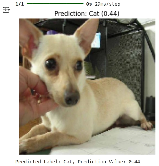
Wait, but that's not a cat...

And you would be correct! Unfortunately, our model can only do so much before it fails against an image input.

If you observe above, it was actually pretty close to predicting a dog, where the prediction value for a dog is greater than 0.5.

The only way we can go from here is to try and fully optimize the next trained model.

This is an example of a scenario called underfitting, where the model failed to learn enough features to make an accurate prediction.

Quick notes before moving on

High accuracy in the training does not necessarily mean that your model will perform well. It could be a scenario called overfitting, meaning your model is memorizing the data too well, to the point that it would do terrible against new data.

Underfitting is the opposite, where it doesn't learn any meaningful patterns in the data.

Optimization

Hyperparameters

Hyperparameters are parameters that control the learning process of the model. Think of it as like configuration settings for the model's learning process.

Altering these hyperparameters would change how the model learns, which influences the final output model. The two most commonly altered hyperparameters for each trained model would be epochs and learning rate.

Epochs is, in simple terms, how many times the model goes through the training process, basically how many laps of trial-and-error it will go through.

Too many epochs can make the model overfit, meaning it fits its given dataset too well.

Too little epochs can make it underfit, meaning it doesn't learn from or doesn't fit its given dataset.

Learning Rate is how fast a model's parameters adjust during each iteration of the optimizer, in this case, the Stochastic Gradient Descent optimizer.

Too high of a learning rate can make the model underfit.
Too low of a learning rate can make the model training very slow.

Model architecture

One of the ways we can do to try and improve future models is by altering its architecture. This is also another type of hyperparameter.

For example, here we added a smaller convolutional layer at the start:

  model = Sequential([
    Conv2D(16, (3,3), activation='relu', input_shape=(150, 150, 3)),
    Conv2D(32, (3,3), activation='relu'),
    MaxPooling2D(2,2),

    Conv2D(64, (3,3), activation='relu'),
    MaxPooling2D(2,2),

    Flatten(),
    Dense(128, activation='relu'),
    Dense(1, activation='sigmoid')  
])

or we could alter it like this:

  model = Sequential([
    Conv2D(16, (3,3), activation='relu', input_shape=(150, 150, 3)),
    MaxPooling2D(2,2),

    Conv2D(32, (3,3), activation='relu'),
    MaxPooling2D(2,2),

    Conv2D(64, (3,3), activation='relu'),
    MaxPooling2D(2,2),

    Flatten(),
    Dense(128, activation='relu'),
    Dense(1, activation='sigmoid')  
])

The possibilities are almost limitless! Do note that this alters the overall way the model actually sees the input, which could actually make the model perform worse.

Image augmentation

Another way to prevent our model from overfitting would be to implement image augmentation.

This is a generalization technique to prevent overfitting by performing random changes to the images.

For example we could:

Zoom into and out the image
Flip the image
Rotate the image
and apply a lot more augmentations

This helps the model adapt to noise that builds up from the background, how the animal is sitting, different lighting, varying angles, and a lot more. Augmentations to the image make it really focus on the important shapes found in the images, making it more adaptable to newer data.

This is somewhat of a double-edged sword as too much augmentations could create even more noise.

Keras actually allows us to do image augmentation using the ImageDataGenerator from earlier.

# COPY OF Data preprocessing with ImageDataGenerator
from tensorflow.keras.preprocessing.image import ImageDataGenerator
import os


directory_for_images = 'data/dogs_vs_cats' # define the parent directory as a variable

# tip from authors: you can see the directory tree if you click on the folder on the left sidebar

train_directory = os.path.join(directory_for_images, 'train') # directory for training data
test_directory = os.path.join(directory_for_images, 'test') # directory for test data


# Image data generator from Keras
# - rescale=1./255 - Divides every pixel value by 255
# - rotation_range=30 - Rotates the image randomly, up to 30 degrees
# - zoom_range=0.2 - Zooms the image in and out by 0.2x
# - horizontal_flip=True - flips the image 50% of the time horizontally
# - vertical_flip=True - flips the image 50% of the time vertically
train_datagen = ImageDataGenerator(
    rescale=1./255,
    rotation_range=30,
    zoom_range=0.2,           # zoom in/out
    horizontal_flip=True,     # flip horizontally
    vertical_flip=True       # flip vertically
)




# Creating the training data generator.
# - train_directory: directory to training data.
# - target_size=(150, 150): Resizes all images to 150x150 pixels.
# - batch_size=32: Loads 32 images per batch.
# - class_mode='binary': For binary classification (Cat vs Dog), returns 0 or 1.
# - subset='training': Uses the training subset as defined by validation_split (80% of the data).
train_generator = train_datagen.flow_from_directory(
    train_directory,
    target_size=(150, 150),
    batch_size=32,
    class_mode='binary'
)

# Creating the validation data generator.
# Same as above, but the directory has changed
val_generator = train_datagen.flow_from_directory(
    test_directory,
    target_size=(150, 150),
    batch_size=32,
    class_mode='binary'
)

# Since we are running a Jupyter notebook over Google Colab,
# running the Training the Model section should just work with the new augmented data if you run this first.

Conclusion

Trying to get a computer to tell the difference between cats and dogs sounds simple, but in reality, it's far from a one-click task. There's a lot that goes into teaching a program to recognize patterns in pictures, from picking the right set of photos, to choosing how many times it should practice, to deciding how much to let it adjust each time. It's a balancing act, and depending on what choices you make, the results can really change.

There are so many knobs and dials to tweak when it comes to training models. You can switch up the dataset, try different numbers of epochs, adjust the learning rate (go fast or take it slow!), or even rethink the model architecture altogether. Want to go deeper? Try throwing in more image augmentation, flip those cats, zoom those dogs, rotate like there’s no tomorrow! Every little change can lead to big discoveries (and possibly better accuracy too). And hey, why stop at just cats and dogs? The world is full of things to classify—muffins vs. chihuahuas, anyone?

If you've made it this far, don't stop here. Keep experimenting, keep tinkering, and most of all, have fun with it. Who says technology can't be playful?