


![[The AI Show Episode 144]: ChatGPT’s New Memory, Shopify CEO’s Leaked “AI First” Memo, Google Cloud Next Releases, o3 and o4-mini Coming Soon & Llama 4’s Rocky Launch](https://www.marketingaiinstitute.com/hubfs/ep%20144%20cover.png)


.jpg?width=1920&height=1920&fit=bounds&quality=70&format=jpg&auto=webp#)


_Olekcii_Mach_Alamy.jpg?width=1280&auto=webp&quality=80&disable=upscale#)


![Apple Drops New Immersive Adventure Episode for Vision Pro: 'Hill Climb' [Video]](https://www.iclarified.com/images/news/97133/97133/97133-640.jpg)
![Most iPhones Sold in the U.S. Will Be Made in India by 2026 [Report]](https://www.iclarified.com/images/news/97130/97130/97130-640.jpg)
![Apple to Shift Robotics Unit From AI Division to Hardware Engineering [Report]](https://www.iclarified.com/images/news/97128/97128/97128-640.jpg)


Building a Logistic Regression Model with Python & Running the Project in Docker: A Hands-On Guide
Building a Logistic Regression Model with Python: A Hands-On Guide Logistic regression is one of the most commonly used machine learning algorithms for classification problems. In this post, we will walk through the steps to implement a simple logistic regression model on the famous Iris dataset, visualize some data characteristics, and save the trained model for future use. Download this Dataset Step 1: Loading the Dataset First, we load the Iris dataset, which is stored in a CSV file. The dataset contains 150 rows and 5 columns, where each row represents a flower sample and includes measurements like Sepal Length, Sepal Width, Petal Length, and Petal Width, along with the species of the flower. from pandas import read_csv filename = "Iris.csv" data = read_csv(filename) Step 2: Displaying Dataset Information After loading the dataset, it's essential to understand its structure. We can check the dataset's shape and preview the first 20 rows to get a feel of the data. print("Shape of the dataset:", data.shape) print("First 20 rows:\n", data.head(20)) Step 3: Visualizing Data with Histograms Before building a model, it's crucial to visualize the data. Histograms give us a quick overview of the distribution of each feature. We plot and save them silently to avoid displaying them in the notebook. from matplotlib import pyplot data.hist() pyplot.savefig("histograms.png") pyplot.close() Step 4: Density Plot for Data Distribution Next, we plot density plots to better understand the distribution of each feature. This can help us detect skewness or identify any patterns that might be useful during training. data.plot(kind='density', subplots=True, layout=(3,3), sharex=False) pyplot.savefig("density_plots.png") pyplot.close() Step 5: Preparing the Data for Training Now, we convert the dataset into a NumPy array and separate the features (the measurements) from the labels (species). This will allow us to feed the data into the logistic regression model. array = data.values X = array[:, 1:5] # Features: Sepal/Petal measurements Y = array[:, 5] # Target: Species Step 6: Splitting the Data We split the data into training (67%) and testing (33%) sets to evaluate our model's performance. The train_test_split function from sklearn handles this. from sklearn.model_selection import train_test_split test_size = 0.33 seed = 7 X_train, X_test, Y_train, Y_test = train_test_split(X, Y, test_size=test_size, random_state=seed) Step 7: Building and Training the Logistic Regression Model We now create a logistic regression model and train it using the training data. We set max_iter=200 to ensure the model has enough iterations to converge. from sklearn.linear_model import LogisticRegression model = LogisticRegression(max_iter=200) model.fit(X_train, Y_train) Step 8: Evaluating Model Accuracy Once the model is trained, we evaluate its performance on the testing set. We calculate the accuracy to see how well the model generalizes. result = model.score(X_test, Y_test) print("Accuracy: {:.2f}%".format(result * 100)) Step 9: Saving the Trained Model Finally, we save the trained model using joblib so we can load it later for predictions without retraining. import joblib joblib.dump(model, "logistic_model.pkl") Running the Project in Docker Prerequisite Download Docker Desktop Run the App Create the Project Structure Create a folder named iris_logistic_regression/ and place the following files inside: iris_logistic_regression/ │ ├── Iris.csv ├── model.py ├── requirements.txt └── Dockerfile Dockerfile code FROM python:3.9-slim RUN pip install pandas scikit-learn matplotlib COPY . . CMD ["python","iris.py"] Build the Docker Image docker build -t iamjabastin/24mcr037-ml:latest . Check the image docker images Push the image docker push iamjabastin/24mcr037-ml Open the Docker Desktop Run the Docker Image Docker Image runs successfully with the output.
Building a Logistic Regression Model with Python: A Hands-On Guide
Logistic regression is one of the most commonly used machine learning algorithms for classification problems. In this post, we will walk through the steps to implement a simple logistic regression model on the famous Iris dataset, visualize some data characteristics, and save the trained model for future use.
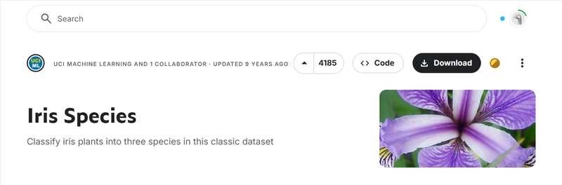
Download this Dataset
Step 1: Loading the Dataset
First, we load the Iris dataset, which is stored in a CSV file. The dataset contains 150 rows and 5 columns, where each row represents a flower sample and includes measurements like Sepal Length, Sepal Width, Petal Length, and Petal Width, along with the species of the flower.
from pandas import read_csv
filename = "Iris.csv"
data = read_csv(filename)
Step 2: Displaying Dataset Information
After loading the dataset, it's essential to understand its structure. We can check the dataset's shape and preview the first 20 rows to get a feel of the data.
print("Shape of the dataset:", data.shape)
print("First 20 rows:\n", data.head(20))
Step 3: Visualizing Data with Histograms
Before building a model, it's crucial to visualize the data. Histograms give us a quick overview of the distribution of each feature. We plot and save them silently to avoid displaying them in the notebook.
from matplotlib import pyplot
data.hist()
pyplot.savefig("histograms.png")
pyplot.close()
Step 4: Density Plot for Data Distribution
Next, we plot density plots to better understand the distribution of each feature. This can help us detect skewness or identify any patterns that might be useful during training.
data.plot(kind='density', subplots=True, layout=(3,3), sharex=False)
pyplot.savefig("density_plots.png")
pyplot.close()
Step 5: Preparing the Data for Training
Now, we convert the dataset into a NumPy array and separate the features (the measurements) from the labels (species). This will allow us to feed the data into the logistic regression model.
array = data.values
X = array[:, 1:5]  # Features: Sepal/Petal measurements
Y = array[:, 5]    # Target: Species
Step 6: Splitting the Data
We split the data into training (67%) and testing (33%) sets to evaluate our model's performance. The train_test_split function from sklearn handles this.
from sklearn.model_selection import train_test_split
test_size = 0.33
seed = 7
X_train, X_test, Y_train, Y_test = train_test_split(X, Y, test_size=test_size, random_state=seed)
Step 7: Building and Training the Logistic Regression Model
We now create a logistic regression model and train it using the training data. We set max_iter=200 to ensure the model has enough iterations to converge.
from sklearn.linear_model import LogisticRegression
model = LogisticRegression(max_iter=200)
model.fit(X_train, Y_train)
Step 8: Evaluating Model Accuracy
Once the model is trained, we evaluate its performance on the testing set. We calculate the accuracy to see how well the model generalizes.
result = model.score(X_test, Y_test)
print("Accuracy: {:.2f}%".format(result * 100))
Step 9: Saving the Trained Model
Finally, we save the trained model using joblib so we can load it later for predictions without retraining.
import joblib
joblib.dump(model, "logistic_model.pkl")
Running the Project in Docker
Prerequisite
- Download Docker Desktop
- Run the App
Create the Project Structure
Create a folder named iris_logistic_regression/ and place the following files inside:
iris_logistic_regression/
│
├── Iris.csv
├── model.py
├── requirements.txt
└── Dockerfile
Dockerfile code
FROM python:3.9-slim

RUN pip install pandas scikit-learn matplotlib

COPY . .

CMD ["python","iris.py"]
Build the Docker Image
docker build -t iamjabastin/24mcr037-ml:latest .
Check the image
docker images
Push the image
docker push iamjabastin/24mcr037-ml
Open the Docker Desktop
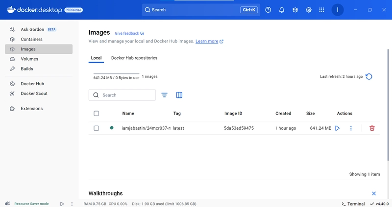
Run the Docker Image
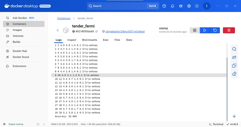
Docker Image runs successfully with the output.