


![[The AI Show Episode 144]: ChatGPT’s New Memory, Shopify CEO’s Leaked “AI First” Memo, Google Cloud Next Releases, o3 and o4-mini Coming Soon & Llama 4’s Rocky Launch](https://www.marketingaiinstitute.com/hubfs/ep%20144%20cover.png)


![GrandChase tier list of the best characters available [April 2025]](https://media.pocketgamer.com/artwork/na-33057-1637756796/grandchase-ios-android-3rd-anniversary.jpg?#)


.png?width=1920&height=1920&fit=bounds&quality=70&format=jpg&auto=webp#)


.webp?#)




![New Beats USB-C Charging Cables Now Available on Amazon [Video]](https://www.iclarified.com/images/news/97060/97060/97060-640.jpg)

![Apple M4 13-inch iPad Pro On Sale for $200 Off [Deal]](https://www.iclarified.com/images/news/97056/97056/97056-640.jpg)


Fusion of Quantum Annealing and Mellin Transform on Berkovich Spaces: A New Perspective on Quantum Computing
Introduction Quantum annealing and non-Archimedean analysis may appear to be disparate mathematical domains, but this article introduces an innovative approach that fuses these concepts. By combining the D-Wave quantum annealing framework with the theory of Mellin transforms on Berkovich analytic spaces, we explore the possibility of analyzing optimization problem solutions from quantum annealing through an entirely new perspective. Representing QUBO Problems on the Berkovich Disk By interpreting Quadratic Unconstrained Binary Optimization (QUBO) problems used in quantum annealing as functions on the Berkovich disk, we can analyze them from a non-Archimedean perspective. # Define a simple QUBO problem Q = {(0, 0): -1, (1, 1): -1, (0, 1): 2} # Create a BinaryQuadraticModel bqm = dimod.BinaryQuadraticModel.from_qubo(Q) # Function to map QUBO to a function on Berkovich disc def qubo_to_berkovich_function(Q, r=1.0): def f(x): if np.isscalar(x): result = 0 for (i, j), coef in Q.items(): result += coef * (x**i) * (x**j) return result else: result = np.zeros_like(x, dtype=float) for (i, j), coef in Q.items(): result += coef * (x**i) * (x**j) return result return f This transformation allows us to handle discrete quantum bit configurations in a continuous function space. Implementation of Mellin Transform on Berkovich Spaces The Mellin transform is an important tool for analyzing the behavior of functions at different scales. By applying the Mellin transform to functions on Berkovich spaces, we can gain new insights into the structure of QUBO problems. def mellin_transform(f, s, a=0, b=1, weights=None): """ Compute the Mellin transform of a function f on [a,b] Parameters: ----------- f : function Function to transform s : complex Transform parameter a, b : float Integration limits (default: [0,1]) weights : function, optional Weight function for the measure """ def integrand(t): if weights is None: return f(t) * (t**(s-1)) else: return f(t) * (t**(s-1)) * weights(t) result, _ = quad(integrand, a, b) return result Solving Problems with D-Wave Quantum Annealing We use actual quantum annealing hardware or simulators to solve QUBO problems and analyze the results. # Create a simulator sampler for testing simulator = neal.SimulatedAnnealingSampler() # Solve using simulator sim_response = simulator.sample(bqm, num_reads=1000) # Try solving using QPU if available try: qpu_sampler = EmbeddingComposite(DWaveSampler()) qpu_response = qpu_sampler.sample(bqm, num_reads=1000, chain_strength=2.0) except Exception as e: print(f"Could not connect to D-Wave QPU: {e}") Analyzing Quantum Annealing Results from a Berkovich Space Perspective By analyzing the energy distribution obtained from quantum annealing from the perspective of Mellin transforms, new features become apparent. # Create a function that represents the energy distribution def energy_distribution(x, energy_values, bins=20): hist, bin_edges = np.histogram(energy_values, bins=bins, density=True) bin_centers = (bin_edges[:-1] + bin_edges[1:]) / 2 # Simple linear interpolation if np.isscalar(x): if x < bin_edges[0] or x > bin_edges[-1]: return 0 idx = np.searchsorted(bin_centers, x) - 1 idx = max(0, min(idx, len(bin_centers)-2)) t = (x - bin_centers[idx]) / (bin_centers[idx+1] - bin_centers[idx]) return hist[idx] * (1-t) + hist[idx+1] * t else: # Vector implementation ... # Compute its Mellin transform mellin_energy = [mellin_transform(energy_dist_func, s, a=min(df.energy), b=max(df.energy)) for s in s_values_energy] Relationship Between Non-Archimedean Seminorms and QUBO Matrices We theoretically explore the relationship between the non-Archimedean properties of Berkovich spaces and QUBO matrices. This may lead to a new understanding of the structure of quantum annealing problems. def analyze_qubo_berkovich_relation(Q): """ Analyze the relationship between QUBO and Berkovich spaces """ # Extract diagonal and off-diagonal terms diagonal = {i: Q.get((i,i), 0) for i in range(max([max(k) for k in Q.keys()])+1)} off_diagonal = {(i,j): Q.get((i,j), 0) for (i,j) in Q.keys() if i != j} # Analytic insights insights = { "diagonal_sum": sum(diagonal.values()), "off_diagonal_sum": sum(off_diagonal.values()), # Further theoretical analysis } return insights Extension to Large-Scale QUBO Problems We extend the Berkovich space and Mellin transform approach to larger QUBO problems, such as
Introduction
Quantum annealing and non-Archimedean analysis may appear to be disparate mathematical domains, but this article introduces an innovative approach that fuses these concepts. By combining the D-Wave quantum annealing framework with the theory of Mellin transforms on Berkovich analytic spaces, we explore the possibility of analyzing optimization problem solutions from quantum annealing through an entirely new perspective.
Representing QUBO Problems on the Berkovich Disk
By interpreting Quadratic Unconstrained Binary Optimization (QUBO) problems used in quantum annealing as functions on the Berkovich disk, we can analyze them from a non-Archimedean perspective.
# Define a simple QUBO problem
Q = {(0, 0): -1, (1, 1): -1, (0, 1): 2}

# Create a BinaryQuadraticModel
bqm = dimod.BinaryQuadraticModel.from_qubo(Q)

# Function to map QUBO to a function on Berkovich disc
def qubo_to_berkovich_function(Q, r=1.0):
    def f(x):
        if np.isscalar(x):
            result = 0
            for (i, j), coef in Q.items():
                result += coef * (x**i) * (x**j)
            return result
        else:
            result = np.zeros_like(x, dtype=float)
            for (i, j), coef in Q.items():
                result += coef * (x**i) * (x**j)
            return result

    return f
This transformation allows us to handle discrete quantum bit configurations in a continuous function space.
Implementation of Mellin Transform on Berkovich Spaces
The Mellin transform is an important tool for analyzing the behavior of functions at different scales. By applying the Mellin transform to functions on Berkovich spaces, we can gain new insights into the structure of QUBO problems.
def mellin_transform(f, s, a=0, b=1, weights=None):
    """
    Compute the Mellin transform of a function f on [a,b]

    Parameters:
    -----------
    f : function
        Function to transform
    s : complex
        Transform parameter
    a, b : float
        Integration limits (default: [0,1])
    weights : function, optional
        Weight function for the measure
    """
    def integrand(t):
        if weights is None:
            return f(t) * (t**(s-1))
        else:
            return f(t) * (t**(s-1)) * weights(t)

    result, _ = quad(integrand, a, b)
    return result
Solving Problems with D-Wave Quantum Annealing
We use actual quantum annealing hardware or simulators to solve QUBO problems and analyze the results.
# Create a simulator sampler for testing
simulator = neal.SimulatedAnnealingSampler()

# Solve using simulator
sim_response = simulator.sample(bqm, num_reads=1000)

# Try solving using QPU if available
try:
    qpu_sampler = EmbeddingComposite(DWaveSampler())
    qpu_response = qpu_sampler.sample(bqm,
                                   num_reads=1000,
                                   chain_strength=2.0)
except Exception as e:
    print(f"Could not connect to D-Wave QPU: {e}")
Analyzing Quantum Annealing Results from a Berkovich Space Perspective
By analyzing the energy distribution obtained from quantum annealing from the perspective of Mellin transforms, new features become apparent.
# Create a function that represents the energy distribution
def energy_distribution(x, energy_values, bins=20):
    hist, bin_edges = np.histogram(energy_values, bins=bins, density=True)
    bin_centers = (bin_edges[:-1] + bin_edges[1:]) / 2

    # Simple linear interpolation
    if np.isscalar(x):
        if x < bin_edges[0] or x > bin_edges[-1]:
            return 0
        idx = np.searchsorted(bin_centers, x) - 1
        idx = max(0, min(idx, len(bin_centers)-2))
        t = (x - bin_centers[idx]) / (bin_centers[idx+1] - bin_centers[idx])
        return hist[idx] * (1-t) + hist[idx+1] * t
    else:
        # Vector implementation
        ...

# Compute its Mellin transform
mellin_energy = [mellin_transform(energy_dist_func, s,
                                 a=min(df.energy),
                                 b=max(df.energy)) for s in s_values_energy]
Relationship Between Non-Archimedean Seminorms and QUBO Matrices
We theoretically explore the relationship between the non-Archimedean properties of Berkovich spaces and QUBO matrices. This may lead to a new understanding of the structure of quantum annealing problems.
def analyze_qubo_berkovich_relation(Q):
    """
    Analyze the relationship between QUBO and Berkovich spaces
    """
    # Extract diagonal and off-diagonal terms
    diagonal = {i: Q.get((i,i), 0) for i in range(max([max(k) for k in Q.keys()])+1)}
    off_diagonal = {(i,j): Q.get((i,j), 0) for (i,j) in Q.keys() if i != j}

    # Analytic insights
    insights = {
        "diagonal_sum": sum(diagonal.values()),
        "off_diagonal_sum": sum(off_diagonal.values()),
        # Further theoretical analysis
    }

    return insights
Extension to Large-Scale QUBO Problems
We extend the Berkovich space and Mellin transform approach to larger QUBO problems, such as graph partitioning.
# Define a larger QUBO problem (e.g., graph partitioning)
def create_graph_partitioning_qubo(n_nodes=4, edge_weights=None):
    """
    Create a QUBO for graph partitioning
    """
    if edge_weights is None:
        # Create a default complete graph
        edge_weights = {(i,j): 1.0 for i in range(n_nodes) for j in range(i+1, n_nodes)}

    # Create QUBO
    Q = {}

    # Add penalty for unbalanced partitions
    for i in range(n_nodes):
        Q[(i,i)] = -1
        for j in range(i+1, n_nodes):
            Q[(i,j)] = 2

    # Add edge weights
    for (i,j), weight in edge_weights.items():
        if i != j:
            Q[(i,j)] = Q.get((i,j), 0) + 2 * weight

    return Q
Conclusion and Future Research Directions
The fusion of quantum annealing and Mellin transforms on Berkovich spaces has the potential to bring new perspectives to both quantum computing and non-Archimedean analysis. Future research directions include:
Further exploration of the relationship between QUBO matrix structures and the characteristics of functions on Berkovich spaces
Feature extraction and solution quality evaluation through Mellin transforms of quantum annealing result distributions
Development of methods for parameter tuning of quantum annealing from a non-Archimedean perspective
Construction of a theoretical framework connecting seminorms on Berkovich spaces with interactions between quantum bits
We hope to explore how this integrative approach may open new avenues for expanding our understanding and application of quantum computing technologies.
References
DOI 10.5281/zenodo.15094922.
DOI 10.5281/zenodo.15111548.
DOI 10.5281/zenodo.15151883.
About the Author
Hello dev.to!