Linear Regression from a high level to code implementation

Regression is simply a statistical process used to understand and model relationship between variables(2 or more) with the goal of Predicting continuous output values using a set of input values Regression can be linear or non-linear Linear Regression is statistical process that models the relationship between a target feature(variable) and independent input feature(s) using a linear equation Or Linear regression is a type of Regression that creates and uses a Linear model to perform it's prediction A model is a simplified (abstract) representation of a complex entity (object) in the real world An Object is anything which can have a defined role to play when solving a problem In our context our Models will be Mathematical equations For a better understanding let's explore Linear Regression from the idea of Covariance and Correlations Covariance is a measure of how two variables change together. More specifically, it tells you whether an increase in one variable will likely result in an increase or decrease in another variable. In simple terms, covariance shows the direction of the relationship between two variables. However, it doesn't provide much information about the strength of that relationship, nor is it easy to interpret in a standardized way because its value depends on the scale of the variables. _mathematically _ the covariance of 2 variables X and Y is given as Cov(X,Y)=1n−1∑i=1n(Xi−Xˉ)(Yi−Yˉ) \text{Cov}(X, Y) = \frac{1}{n-1} \displaystyle\sum_{i=1}^{n} (X_i - \bar{X})(Y_i - \bar{Y}) Cov(X,Y)=n−11i=1∑n(Xi−Xˉ)(Yi−Yˉ) Covariance can be positive, zero, or negative positive:both variable increase together negative:one increases as the other decreases zero:no predictable relationship between the variables. While Covariance tells us whether two variables move together, it doesn't standardize how strongly they move together. This is where Correlations comes in. By dividing the covariance of two variables by the product of their standard deviations, we get a dimensionless measure called the correlation coefficient (usually denoted as r): r=Cov(X,Y)σXσY, andσX=1n−1∑i=1n(Xi−Xˉ)2 r = \frac{\text{Cov}(X, Y)}{\sigma_X \sigma_Y}, \text{ }{ and }{} \sigma_X = \sqrt{\frac{1}{n - 1} \sum_{i=1}^{n} (X_i - \bar{X})^2} r=σXσYCov(X,Y), andσX=n−11i=1∑n(Xi−Xˉ)2 A simple example in python # Sample data x = [2, 4, 6, 8, 10] y = [1, 3, 5, 7, 9] # Function to compute mean def mean(data): return sum(data) / len(data) # Function to compute covariance def covariance(x, y): x_mean = mean(x) y_mean = mean(y) return sum((xi - x_mean) * (yi - y_mean) for xi, yi in zip(x, y)) / len(x) # Function to compute standard deviation def stddev(data): data_mean = mean(data) return (sum((x - data_mean) 2 for x in data) / len(data)) 0.5 # Function to compute correlation def correlation(x, y): return covariance(x, y) / (stddev(x) * stddev(y)) # Output print("Covariance:", round(covariance(x, y), 4)) print("Correlation:", round(correlation(x, y), 4)) # Plot plt.figure(figsize=(6, 4)) plt.scatter(x, y, color='blue', label='Data points') plt.plot(x, y, color='green', linestyle='--', label='Trend line') # Add text info plt.title(f"Scatter Plot\nCovariance: {round(cov, 2)} | Correlation: {round(corr, 2)}") plt.xlabel('X') plt.ylabel('Y') plt.legend() plt.grid(True) plt.tight_layout() plt.show() example with a csv file import pandas as pd import matplotlib.pyplot as plt # Load the CSV file df = pd.read_csv('data.csv') # Make sure this file exists in your working directory # Extract two columns x = df['height'] y = df['weight'] # Compute covariance and correlation cov = df[['height', 'weight']].cov().iloc[0, 1] corr = df[['height', 'weight']].corr().iloc[0, 1] # Print results print(f"Covariance: {round(cov, 4)}") print(f"Correlation: {round(corr, 4)}") # Plot plt.figure(figsize=(6, 4)) plt.scatter(x, y, color='teal', label='Data Points') plt.plot(x, y, color='coral', linestyle='--', label='Trend Line') plt.title(f"Height vs Weight\nCovariance: {round(cov, 2)} | Correlation: {round(corr, 2)}") plt.xlabel('Height') plt.ylabel('Weight') plt.legend() plt.grid(True) plt.tight_layout() plt.show() In a nutshel Correlation coefficient (r) describes the strength and direction of the relationship between two or more variables in a standard way that is independent of their respective units of measurement. Meanwhile the Covariance which does a pretty good job for the same task is highly affected by the units of measurement of the variables in concern. Now that we understand covariance and the correlation coefficient, we are ready to step into linear regression—a cornerstone of predictive modeling. While the correlation coefficient(r) tells us how strong the relationship is between two variables, it doesn’t tell us the exact nature of the relationship. This is where linear regression comes in. Linear regression aims to mode

Apr 14, 2025 - 19:24

Linear Regression from a high level to code implementation

Regression is simply a statistical process used to understand and model relationship between variables(2 or more) with the goal of Predicting continuous output values using a set of input values

Regression can be linear or non-linear

Linear Regression is statistical process that models the relationship between a target feature(variable) and independent input feature(s)
using a linear equation

Or
Linear regression is a type of Regression that creates and uses a Linear model to perform it's prediction

A model is a simplified (abstract) representation of a complex entity (object) in the real world

An Object is anything which can have a defined role to play when solving a problem

In our context our Models will be Mathematical equations
For a better understanding let's explore Linear Regression from the idea of Covariance and Correlations

Covariance is a measure of how two variables change together. More specifically, it tells you whether an increase in one variable will likely result in an increase or decrease in another variable. In simple terms, covariance shows the direction of the relationship between two variables. However, it doesn't provide much information about the strength of that relationship, nor is it easy to interpret in a standardized way because its value depends on the scale of the variables.
_mathematically _ the covariance of 2 variables X and Y is given as

\text{Cov}(X, Y) = \frac{1}{n-1} \displaystyle\sum_{i=1}^{n} (X_i - \bar{X})(Y_i - \bar{Y})

Covariance can be positive, zero, or negative
positive:both variable increase together
negative:one increases as the other decreases
zero:no predictable relationship between the variables.

While Covariance tells us whether two variables move together, it doesn't standardize how strongly they move together. This is where Correlations comes in. By dividing the covariance of two variables by the product of their standard deviations, we get a dimensionless measure called the correlation coefficient (usually denoted as r):

\frac{\text{Cov}(X, Y)}{\sigma_X \sigma_Y}, \text{ }{ and }{} \sigma_X = \sqrt{\frac{1}{n - 1} \sum_{i=1}^{n} (X_i - \bar{X})^2}

A simple example in python

# Sample data
x = [2, 4, 6, 8, 10]
y = [1, 3, 5, 7, 9]

# Function to compute mean
def mean(data):
    return sum(data) / len(data)

# Function to compute covariance
def covariance(x, y):
    x_mean = mean(x)
    y_mean = mean(y)
    return sum((xi - x_mean) * (yi - y_mean) for xi, yi in zip(x, y)) / len(x)

# Function to compute standard deviation
def stddev(data):
    data_mean = mean(data)
    return (sum((x - data_mean) ** 2 for x in data) / len(data)) ** 0.5

# Function to compute correlation
def correlation(x, y):
    return covariance(x, y) / (stddev(x) * stddev(y))

# Output
print("Covariance:", round(covariance(x, y), 4))
print("Correlation:", round(correlation(x, y), 4))

# Plot
plt.figure(figsize=(6, 4))
plt.scatter(x, y, color='blue', label='Data points')
plt.plot(x, y, color='green', linestyle='--', label='Trend line')

# Add text info
plt.title(f"Scatter Plot\nCovariance: {round(cov, 2)} | Correlation: {round(corr, 2)}")
plt.xlabel('X')
plt.ylabel('Y')
plt.legend()
plt.grid(True)
plt.tight_layout()
plt.show()

example with a csv file

import pandas as pd
import matplotlib.pyplot as plt

# Load the CSV file
df = pd.read_csv('data.csv')  # Make sure this file exists in your working directory

# Extract two columns
x = df['height']
y = df['weight']

# Compute covariance and correlation
cov = df[['height', 'weight']].cov().iloc[0, 1]
corr = df[['height', 'weight']].corr().iloc[0, 1]

# Print results
print(f"Covariance: {round(cov, 4)}")
print(f"Correlation: {round(corr, 4)}")

# Plot
plt.figure(figsize=(6, 4))
plt.scatter(x, y, color='teal', label='Data Points')
plt.plot(x, y, color='coral', linestyle='--', label='Trend Line')

plt.title(f"Height vs Weight\nCovariance: {round(cov, 2)} | Correlation: {round(corr, 2)}")
plt.xlabel('Height')
plt.ylabel('Weight')
plt.legend()
plt.grid(True)
plt.tight_layout()
plt.show()

In a nutshel Correlation coefficient (r) describes the strength and direction of the relationship between two or more variables in a standard way that is independent of their respective units of measurement. Meanwhile the Covariance which does a pretty good job for the same task is highly affected by the units of measurement of the variables in concern.

Now that we understand covariance and the correlation coefficient, we are ready to step into linear regression—a cornerstone of predictive modeling.

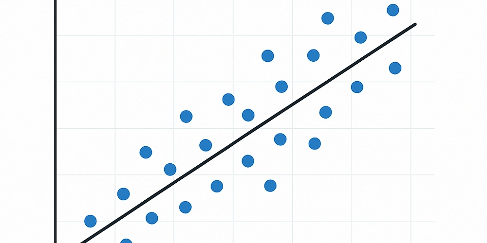
While the correlation coefficient(r) tells us how strong the relationship is between two variables, it doesn’t tell us the exact nature of the relationship. This is where linear regression comes in.

Linear regression aims to model the relationship between an independent variable,(X) and a dependent variable (y) by fitting a straight line:

$y = m x + b$

Where:

y is the predicted value (dependent variable),
X is the input feature (independent variable),
m is the slope of the line,
b is the y-intercept.

Our goal is to find the values of m and b such that the line "best fits" the data.

Deriving the Best Fit Line

To compute the slope m and intercept b, we use the least squares method. This method minimizes the sum of the squared differences between the observed values and the predicted values.

Slope (m):

\frac{\sum (x_i - \bar{x})(y_i - \bar{y})}{\sum (x_i - \bar{x})^2}

You might recognize the numerator—it's the covariance between X and y, while the denominator is the variance of X.

So, another way to write it is:

\frac{\text{Cov}(x, y)}{\text{Var}(x)}

Intercept (b):

\bar{y} - m\bar{x}

Where:

$Xˉ\bar{X}$ is the mean of X,
$yˉ\bar{y}$ is the mean of y.

Intuition Behind the Line

The line $y = m x + c$ passes through the point ( $Xˉ\bar{X}$ , $yˉ\bar{y}$ )That is, the line always intersects the mean of the data.

Also, the slope (m) tells us how much y changes for a unit increase in X. A positive slope means a positive relationship, and vice versa.

Implementing Linear Regression in Code (No Libraries)
Let’s implement this in pure Python, so we understand every step.

# Sample data
x = [1, 2, 3, 4, 5]
y = [2, 4, 5, 4, 5]

# Step 1: Calculate means
x_mean = sum(x) / len(x)
y_mean = sum(y) / len(y)

# Step 2: Calculate slope (m)
numerator = sum((xi - x_mean) * (yi - y_mean) for xi, yi in zip(x, y))
denominator = sum((xi - x_mean) ** 2 for xi in x)
m = numerator / denominator

# Step 3: Calculate intercept (b)
b = y_mean - m * x_mean

# Final equation
print(f"Regression line: y = {m:.2f}x + {b:.2f}")

Evaluation Metrics for Linear Regression

Once you've trained your regression model, it's crucial to assess how well it's performing. Below are the most widely used metrics for evaluating linear regression.

1. Mean Absolute Error (MAE)

Mean Absolute Error measures the average of the absolute differences between predicted and actual values.

MAE=1n∑i=1n∣yi−y^i∣ \text{MAE} = \frac{1}{n} \sum_{i=1}^{n} \left| y_i - \hat{y}_i \right|

$yi\text{y}_i$ = actual value
$y^i\hat{y}_i$ = predicted value
n = number of data points

It gives a linear score, meaning all errors are weighted equally.

2. Mean Squared Error (MSE)

Mean Squared Error measures the average of the squared differences between predicted and actual values.

MSE=1n∑i=1n(yi−y^i)2 \text{MSE} = \frac{1}{n} \sum_{i=1}^{n} (y_i - \hat{y}_i)^2

Squaring emphasizes larger errors more than smaller ones, making this a sensitive metric to outliers.

3. Root Mean Squared Error (RMSE)

RMSE is simply the square root of MSE. It brings the error metric back to the original unit of the output variable.

RMSE=1n∑i=1n(yi−y^i)2 \text{RMSE} = \sqrt{ \frac{1}{n} \sum_{i=1}^{n} (y_i - \hat{y}_i)^2 }

4. R-squared (Coefficient of Determination)

R-squared () represents the proportion of the variance in the dependent variable that is predictable from the independent variable(s).

R2=1−∑i=1n(yi−y^i)2∑i=1n(yi−yˉ)2 R^2 = 1 - \frac{ \sum_{i=1}^{n} (y_i - \hat{y}i)^2 }{ \sum{i=1}^{n} (y_i - \bar{y})^2 }

Where:

$yˉ\bar{y}$ is the mean of the actual values.

An $R^2$ of:

1.0 means perfect prediction,
0 means no better than predicting the mean,
Negative values can occur when the model performs worse than a horizontal line.

Summary

Metric	Description	Sensitive to Outliers
MAE	Average absolute error	No
MSE	Average squared error	Yes
RMSE	Square root of MSE	Yes
$R^2$	Proportion of explained variance	No (but informative)

Choose the metric that aligns best with your business goals and sensitivity to error types.

Metric evaluation in python

import numpy as np
from sklearn.metrics import mean_absolute_error, mean_squared_error, r2_score

# Actual and predicted values
y_true = np.array([3, -0.5, 2, 7])
y_pred = np.array([2.5, 0.0, 2, 8])

# --- Using NumPy (manual calculations) ---

# MAE
mae = np.mean(np.abs(y_true - y_pred))

# MSE
mse = np.mean((y_true - y_pred)**2)

# RMSE
rmse = np.sqrt(mse)

# R-squared
ss_res = np.sum((y_true - y_pred) ** 2)
ss_tot = np.sum((y_true - np.mean(y_true)) ** 2)
r2 = 1 - (ss_res / ss_tot)

print("Manual Calculation:")
print(f"MAE: {mae:.3f}")
print(f"MSE: {mse:.3f}")
print(f"RMSE: {rmse:.3f}")
print(f"R²: {r2:.3f}")

# --- Using Scikit-learn (recommended for real-world use) ---

mae_sk = mean_absolute_error(y_true, y_pred)
mse_sk = mean_squared_error(y_true, y_pred)
rmse_sk = mean_squared_error(y_true, y_pred, squared=False)  # RMSE directly
r2_sk = r2_score(y_true, y_pred)

print("\nUsing Scikit-learn:")
print(f"MAE: {mae_sk:.3f}")
print(f"MSE: {mse_sk:.3f}")
print(f"RMSE: {rmse_sk:.3f}")
print(f"R²: {r2_sk:.3f}")