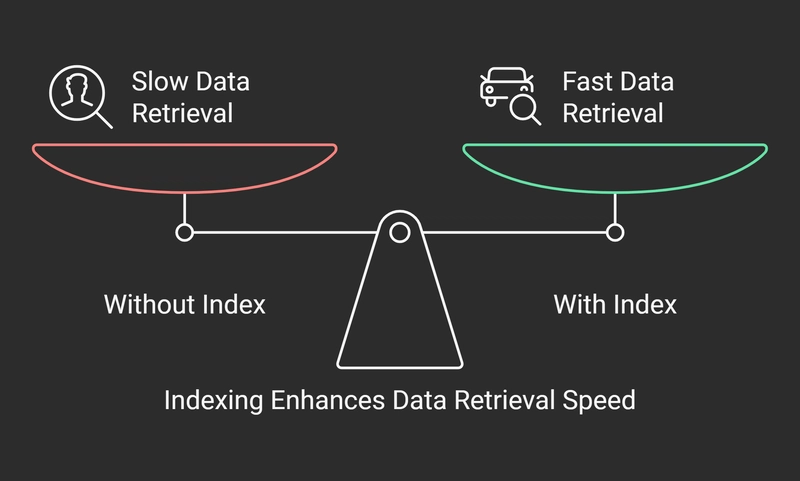
Mastering Database Indexing: Faster Data Access Made Simple!

Imagine you're at a supermarket looking for "chocolate cookies." Would you: Check every aisle one by one? Use the signs above each aisle to go directly to "Snacks & Cookies"? Obviously!, you’d use the signs—that’s exactly what database indexing does for your data! Instead of checking every row in a database, indexing helps the system quickly find the information you need. In this blog, we’ll explore the basics of database indexing, its impact on performance, and how it works using simple, real-life examples, code demos, and visuals. Let's dive in! What is Database Indexing? Imagine a huge database as a giant list of records. Searching through this list without an index is like looking for a needle in a haystack—you’d have to check each record one by one. But with an index, it’s like having a roadmap that shows you exactly where to look! An index in a database is a special data structure that stores pointers to the actual data in a way that makes retrieving information much faster. It's like a catalog that helps you find what you're looking for without scanning everything. Real-Life Example: Finding a Customer’s Order Let’s say you run an e-commerce website, and you need to find a customer’s order. Your database might look like this: Order ID Customer Name Product Amount 3 Alice Smartphone $500 1 Bob Laptop $1200 2 Charlie Headphones $150 4 Alice Tablet $300 5 David Camera $700 6 Eve Watch $200 7 Bob Keyboard $100 8 Frank Monitor $400 9 Charlie Charger $50 10 David Laptop Stand $30 Now, imagine you want to search for "Charlie’s" order. Without an index, the database would scan every row to find "Charlie." This can be slow, especially with a large dataset. But if we create an index on the Customer Name column, the database can quickly find "Charlie" without checking every row. Sorted Reference Table Example The index on Customer Name might look like this: Customer Name Order ID Alice 3, 4 Bob 1, 7 Charlie 2, 9 David 5, 10 Eve 6 Frank 8 Now, instead of scanning all records, the database looks up "Charlie" in the index and directly fetches his order IDs, making the query much faster! Types of Indexing Structures: B-Tree and B+ Tree Modern databases use advanced indexing structures like B-Trees and B+ Trees to organize data efficiently. B-Tree Index A B-Tree (Balanced Tree) stores both keys (values being indexed) and data in its nodes. The tree is balanced, which means that all leaf nodes are at the same depth, ensuring quick access. Example: Searching for "Charlie" in a B-Tree means traversing a few nodes until you find the data. Bob / \ Alice Charlie B+ Tree Index A B+ Tree is similar to the B-Tree, but it stores only keys in the internal nodes, while all data is kept in the leaf nodes. The leaf nodes are also linked, making range queries much more efficient. Example: With a B+ Tree, finding all customers whose names start with "C" is quick because all the relevant data is stored in linked leaf nodes. Bob / \ Alice Charlie --> Leaf Node The key difference between B-Trees and B+ Trees is that B+ Trees allow for faster range queries, making them the preferred choice in many modern databases. Full Tree Example with More Complexity Let’s dive deeper into a more complex example with a B-Tree and B+ Tree, both of which are commonly used for indexing. B-Tree Example Consider the following dataset of customer names and their order IDs: Customer Name Order ID Alice 3 Bob 1 Charlie 2 David 5 Eve 6 Frank 4 Grace 7 We’ll create a B-Tree index for the Customer Name field. Insert 'Alice': Alice is placed at the root. Insert 'Bob': Bob is smaller than Alice, so it goes to the left. Insert 'Charlie': Charlie is placed on the right of Alice. Insert 'David': David fits in between Charlie and Eve, so it goes to the right. Insert 'Eve': Eve fits between David and Frank, so it goes on the right side. Here’s how the B-Tree would look after inserting all elements: Alice / \ Bob Charlie / \ David Eve / \ Frank Grace In this tree, you can see that if you want to search for "David", you start at the root, then go to the right subtree, and finally find the node. B+ Tree Example A B+ Tree is more efficient for range queries. In a B+ Tree, only leaf nodes contain data, and the internal nodes contain keys. All leaf nodes are also linked, making range queries much more efficient. Let’s use the same dataset for a B+ Tree: Customer Name Order ID Alice 3 Bob 1 Charlie 2 David 5 Eve 6 Frank 4 Grace 7 The B+ Tree would look like this: [Charlie] / \ [Bob] [

Apr 2, 2025 - 20:05

Mastering Database Indexing: Faster Data Access Made Simple!

Imagine you're at a supermarket looking for "chocolate cookies." Would you:

Check every aisle one by one?
Use the signs above each aisle to go directly to "Snacks & Cookies"?

Obviously!, you’d use the signs—that’s exactly what database indexing does for your data! Instead of checking every row in a database, indexing helps the system quickly find the information you need. In this blog, we’ll explore the basics of database indexing, its impact on performance, and how it works using simple, real-life examples, code demos, and visuals. Let's dive in!

What is Database Indexing?

Imagine a huge database as a giant list of records. Searching through this list without an index is like looking for a needle in a haystack—you’d have to check each record one by one. But with an index, it’s like having a roadmap that shows you exactly where to look!

An index in a database is a special data structure that stores pointers to the actual data in a way that makes retrieving information much faster. It's like a catalog that helps you find what you're looking for without scanning everything.

Real-Life Example: Finding a Customer’s Order

Let’s say you run an e-commerce website, and you need to find a customer’s order. Your database might look like this:

Order ID	Customer Name	Product	Amount
3	Alice	Smartphone	$500
1	Bob	Laptop	$1200
2	Charlie	Headphones	$150
4	Alice	Tablet	$300
5	David	Camera	$700
6	Eve	Watch	$200
7	Bob	Keyboard	$100
8	Frank	Monitor	$400
9	Charlie	Charger	$50
10	David	Laptop Stand	$30

Now, imagine you want to search for "Charlie’s" order. Without an index, the database would scan every row to find "Charlie." This can be slow, especially with a large dataset.

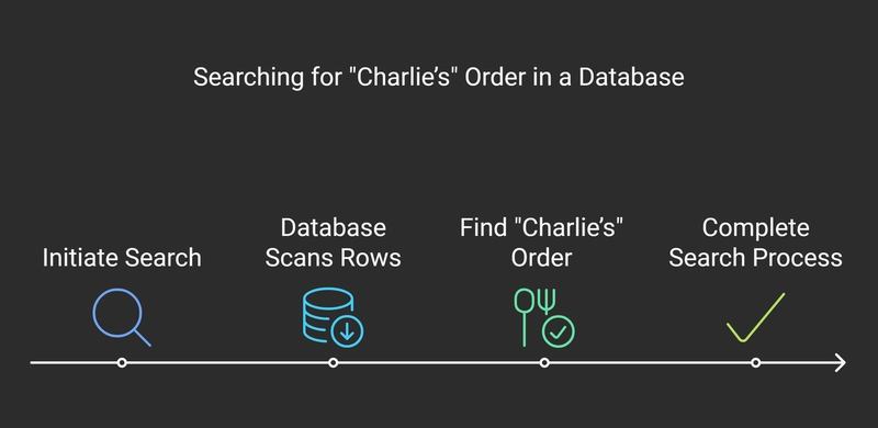
But if we create an index on the Customer Name column, the database can quickly find "Charlie" without checking every row.

Sorted Reference Table Example

The index on Customer Name might look like this:

Customer Name	Order ID
Alice	3, 4
Bob	1, 7
Charlie	2, 9
David	5, 10
Eve	6
Frank	8

Now, instead of scanning all records, the database looks up "Charlie" in the index and directly fetches his order IDs, making the query much faster!

Types of Indexing Structures: B-Tree and B+ Tree

Modern databases use advanced indexing structures like B-Trees and B+ Trees to organize data efficiently.

B-Tree Index

A B-Tree (Balanced Tree) stores both keys (values being indexed) and data in its nodes. The tree is balanced, which means that all leaf nodes are at the same depth, ensuring quick access.

Example: Searching for "Charlie" in a B-Tree means traversing a few nodes until you find the data.

        Bob
       /   \
   Alice   Charlie

B+ Tree Index

A B+ Tree is similar to the B-Tree, but it stores only keys in the internal nodes, while all data is kept in the leaf nodes. The leaf nodes are also linked, making range queries much more efficient.

Example: With a B+ Tree, finding all customers whose names start with "C" is quick because all the relevant data is stored in linked leaf nodes.

        Bob
       /   \
   Alice   Charlie --> Leaf Node

The key difference between B-Trees and B+ Trees is that B+ Trees allow for faster range queries, making them the preferred choice in many modern databases.

Full Tree Example with More Complexity

Let’s dive deeper into a more complex example with a B-Tree and B+ Tree, both of which are commonly used for indexing.

B-Tree Example

Consider the following dataset of customer names and their order IDs:

Customer Name	Order ID
Alice	3
Bob	1
Charlie	2
David	5
Eve	6
Frank	4
Grace	7

We’ll create a B-Tree index for the Customer Name field.

Insert 'Alice': Alice is placed at the root.
Insert 'Bob': Bob is smaller than Alice, so it goes to the left.
Insert 'Charlie': Charlie is placed on the right of Alice.
Insert 'David': David fits in between Charlie and Eve, so it goes to the right.
Insert 'Eve': Eve fits between David and Frank, so it goes on the right side.

Here’s how the B-Tree would look after inserting all elements:

            Alice
          /       \
      Bob          Charlie
                     /      \
                 David      Eve
                             /   \
                          Frank  Grace

In this tree, you can see that if you want to search for "David", you start at the root, then go to the right subtree, and finally find the node.

B+ Tree Example

A B+ Tree is more efficient for range queries. In a B+ Tree, only leaf nodes contain data, and the internal nodes contain keys. All leaf nodes are also linked, making range queries much more efficient.

Let’s use the same dataset for a B+ Tree:

Customer Name	Order ID
Alice	3
Bob	1
Charlie	2
David	5
Eve	6
Frank	4
Grace	7

The B+ Tree would look like this:

         [Charlie]
        /         \
    [Bob]        [David]
       |            |   
    [Alice]      [Eve] --> Linked to Next Leaf
                   /   \
               [Frank] [Grace]

In this structure, only leaf nodes store the actual data, while internal nodes only store the keys. Notice how the leaf nodes are linked, allowing you to easily perform range queries (e.g., find all orders from "Charlie" to "Grace").

Key Differences Between B-Tree and B+ Tree

Feature	B-Tree	B+ Tree
Data Storage	Data in both internal and leaf nodes	Data only in leaf nodes
Internal Nodes	Store both keys and data	Store only keys
Leaf Node Linking	No	Yes, linked leaf nodes
Best Use Case	Point queries	Range queries, large data sets

Impact of Indexing on Read vs. Write Operations

Read Operations (Queries)

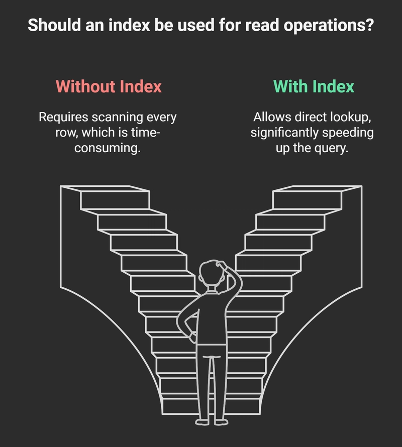
Indexes are designed to speed up read operations. When you query the database, it uses the index to jump directly to the relevant data, saving time.

Without Index: Searching for "Charlie" would require scanning every row in the table.
With Index: The database looks up "Charlie" in the index, making the query faster.

For example, if you're searching for a customer by name in a large table, without an index, the database needs to check every row, which can be slow. But with an index, the search is much faster as it directly finds the location of the data in a sorted structure.

Write Operations (Insert, Update, Delete)

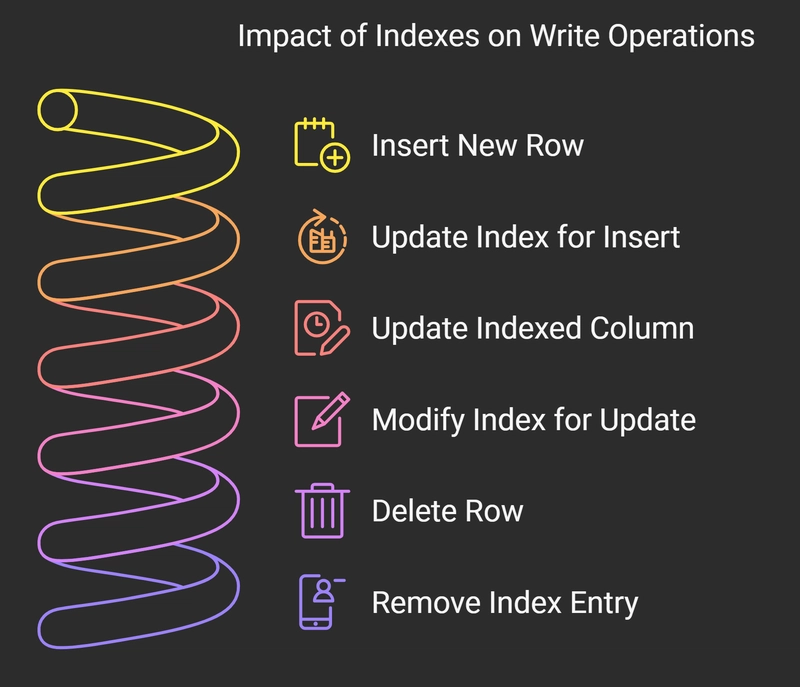
While indexes improve read performance, they can slow down write operations. When a new row is inserted, updated, or deleted, the index must also be updated to reflect the changes in the data.

Insert: When a new row is inserted, the database not only inserts the row into the table but also updates the index, which takes extra time.
Update: If an indexed column is updated, the index must be modified to reflect the new value, which adds overhead to the update process.
Delete: When a row is deleted, the corresponding entry in the index must also be removed, adding extra processing time.

In summary, while indexes significantly speed up read queries, they add overhead to write operations, especially in tables with multiple indexes or large datasets.

Code Example: Indexing in SQL (With Detailed Analysis)

Indexes significantly improve query performance by allowing the database to find records quickly instead of scanning the entire table. However, they come with trade-offs, especially for write operations.

In this section, we will:

Create a table
Insert sample data
Compare queries with and without an index
Analyze query execution plans
Discuss the impact of indexes on different operations

1. Creating a Sample Table

Let's create a customers table with a few columns.

CREATE TABLE customers (
    id SERIAL PRIMARY KEY,
    name VARCHAR(100),
    email VARCHAR(100) UNIQUE,
    city VARCHAR(50)
);

id: Primary key (automatically indexed).
name: A column we may index later.
email: Unique constraint (automatically indexed).
city: A regular column.

2. Inserting Sample Data

To make the performance impact visible, let's insert 1 million records.

DO $$ 
BEGIN 
    FOR i IN 1..1000000 LOOP
        INSERT INTO customers (name, email, city)
        VALUES (
            'Customer' || i,
            'customer' || i || '@example.com',
            CASE WHEN i % 3 = 0 THEN 'New York'
                 WHEN i % 3 = 1 THEN 'Los Angeles'
                 ELSE 'Chicago'
            END
        );
    END LOOP;
END $$;

This Script:

Inserts 1 million rows into the customers table.
Generates unique names (Customer1, Customer2, ...).
Ensures unique emails (customer1@example.com, customer2@example.com, ...).
Randomly assigns a city (New York, Los Angeles, Chicago).

3. Query Without an Index

Let's search for a customer without an index.

EXPLAIN ANALYZE SELECT * FROM customers WHERE name = 'Customer500000';

Expected Output (Without Index)

Seq Scan on customers  (cost=0.00..43125.00 rows=1 width=68)
   Filter: (name = 'Customer500000'::text)
   Rows Removed by Filter: 999999
   Planning Time: 0.125 ms
   Execution Time: 2034.45 ms

Seq Scan → Scans every row.
Rows Removed → Checks all 1 million rows.
Execution Time → ~2 seconds for one query. This is highly inefficient.

4. Creating an Index

Let's add an index on the name column.

CREATE INDEX idx_customer_name ON customers(name);

Now, rerun the query:

EXPLAIN ANALYZE SELECT * FROM customers WHERE name = 'Customer500000';

Expected Output (With Index)

Index Scan using idx_customer_name on customers  (cost=0.42..8.44 rows=1 width=68)
   Index Cond: (name = 'Customer500000'::text)
   Planning Time: 0.095 ms
   Execution Time: 0.135 ms

What Improved?
✅ Index Scan → Uses the index instead of scanning all rows.
✅ Execution Time → Reduced from 2 seconds to 0.1 ms → HUGE improvement!

5. Impact on Insert, Update, and Delete

5.1 Insert Performance

EXPLAIN ANALYZE INSERT INTO customers (name, email, city) 
VALUES ('NewCustomer', 'newcustomer@example.com', 'Boston');

Expected Output (With Index)

Insert on customers  (cost=0.00..0.01 rows=1 width=0)
   Execution Time: 0.455 ms

Inserts are slightly slower because the database updates the index.

5.2 Update Performance

EXPLAIN ANALYZE UPDATE customers SET city = 'San Francisco' WHERE name = 'Customer500000';

Expected Output

Index Scan using idx_customer_name on customers  (cost=0.42..8.44 rows=1 width=68)
   Index Cond: (name = 'Customer500000'::text)
   Execution Time: 0.225 ms

Finding the record is fast due to the index.
If updating an indexed column, the database rebuilds the index, making it slower.

5.3 Delete Performance

EXPLAIN ANALYZE DELETE FROM customers WHERE name = 'Customer500000';

Expected Output

Index Scan using idx_customer_name on customers  (cost=0.42..8.44 rows=1 width=68)
   Index Cond: (name = 'Customer500000'::text)
   Execution Time: 0.290 ms

Fast lookup, but removing from index adds overhead.

6. Dropping an Index

If indexing slows down inserts/updates, remove it.

DROP INDEX idx_customer_name;

After dropping the index:

Searches become slower.
Inserts, updates, and deletes become faster.

7. When to Use Indexes?

Scenario	Use an Index?
Frequently searching a column	✅ Yes
Sorting a large dataset	✅ Yes
Joining large tables	✅ Yes
Frequently updating a column	❌ No
High insert/delete operations	❌ No

Best Practices

Index columns used in WHERE, ORDER BY, and JOIN.
Avoid indexing frequently updated columns.
Limit the number of indexes.
Use Composite Indexes if filtering by multiple columns.

Example of a Composite Index:

CREATE INDEX idx_name_city ON customers(name, city);

Now, searches on both name and city are optimized.

8. Summary

Operation	Without Index	With Index
SELECT	Slow (Full Scan)	Fast (Index Scan)
INSERT	Fast	Slightly Slower
UPDATE (Indexed Column)	Fast	Slower (Index Must Update)
DELETE	Fast	Slightly Slower

Indexes boost query performance but come at the cost of slower writes. The key is balancing speed vs. overhead.

Types of Indexes (Other than B-Tree/B+ Tree)

Hash Indexing

A hash index is an indexing technique that uses a hash table. It's often used for equality comparisons (=) rather than range queries.

Example
If you're looking for a record where the value of a column equals a specific value, hash indexing can be very efficient:

CREATE INDEX idx_hash_email ON users USING HASH(email);

However, hash indexing is not useful for range queries (BETWEEN, >, <), and some databases (like MySQL) do not support hash indexes for general use.

Full-Text Indexing

Full-text indexing is used to optimize search queries on large text fields. In full-text search, the text is tokenized, and each token is indexed separately.

Example (MySQL):

CREATE FULLTEXT INDEX idx_fulltext_desc ON products(description);

This would optimize queries like:

SELECT * FROM products WHERE MATCH(description) AGAINST ('laptop');

Spatial Indexing

Spatial indexing is used to optimize queries on geometric or geographic data, like points, lines, or polygons.

Example (PostgreSQL with PostGIS):

CREATE INDEX idx_gist_location ON locations USING GIST (geom);

Indexing Strategies

Composite Indexes

A composite index is an index on multiple columns, which is helpful when queries filter by multiple columns.

Example:

CREATE INDEX idx_composite_name_age ON users(name, age);

This index will optimize queries like:

SELECT * FROM users WHERE name = 'John' AND age = 30;

Partial Indexes

Partial indexes index only a subset of the data, which can be useful for reducing index size and increasing performance for specific queries.

Example:

CREATE INDEX idx_partial_active_users ON users(name) WHERE is_active = 1;

This index would be useful for queries like:

SELECT * FROM users WHERE is_active = 1 AND name = 'John';

Unique Indexes

A unique index ensures that all the values in the indexed columns are distinct.

Example:

CREATE UNIQUE INDEX idx_unique_email ON users(email);

This would enforce that no two users can have the same email address.

Index Maintenance

Index Fragmentation

Indexes can become fragmented as rows are added, updated, or deleted. Fragmentation can reduce performance, and indexes might need to be rebuilt periodically.

In PostgreSQL:

REINDEX INDEX idx_name;

In MySQL:

OPTIMIZE TABLE users;

Rebuilding and Dropping Indexes

Indexes might need to be rebuilt or dropped when they are no longer needed.

Example (Rebuild Index):

ALTER INDEX idx_name REBUILD;

Performance Implications

Query Optimization

Indexes help the database engine find rows more efficiently. The optimizer decides whether to use an index based on factors like query complexity, index statistics, and available indexes.

Example:
A query without an index might require scanning the entire table (a full table scan), while an indexed query will only look at the rows that match the index criteria.

SELECT * FROM products WHERE category = 'electronics';

If there's an index on category, the database can jump directly to the relevant rows.

Cost of Indexing

While indexes speed up read operations, they slow down write operations because the index must be updated every time the table data changes. The trade-off must be considered based on the application’s needs.

Example:
If a table frequently experiences INSERT, UPDATE and DELETE operations, adding too many indexes can degrade performance due to the extra overhead in maintaining those indexes.

Covering Indexes

A covering index is an index that contains all the columns needed for a query, so the database can satisfy the query using only the index (without needing to access the table).

Example:

CREATE INDEX idx_covering ON orders(order_id, customer_id, total_amount);

For a query like:

SELECT order_id, total_amount FROM orders WHERE customer_id = 123;

If the idx_covering index includes both order_id, customer_id and total_amount the query can be satisfied directly by the index.

Database-Specific Indexing Features

PostgreSQL

GiST Indexes (Generalized Search Tree): A versatile indexing method used for various data types like geometric and full-text data.

CREATE INDEX idx_gist_geom ON places USING GiST (location);

GIN Indexes (Generalized Inverted Index): Useful for full-text search and array data.

CREATE INDEX idx_gin_tags ON posts USING GIN (tags);

MySQL

InnoDB vs. MyISAM: InnoDB uses clustered indexes (the table data is stored in the index), while MyISAM uses non-clustered indexes.

CREATE INDEX idx_name_age ON users(name, age) USING BTREE;

SQL Server

Indexed Views: A feature in SQL Server where views can be indexed for performance optimization.

CREATE VIEW vw_sales_summary AS
  SELECT product_id, SUM(sales_amount)
  FROM sales
  GROUP BY product_id;

CREATE UNIQUE CLUSTERED INDEX idx_sales_summary ON vw_sales_summary (product_id);

Indexing and Normalization

Normalization

In normalized databases, indexes optimize queries by providing fast access paths to specific data points, such as foreign key relationships.

Example:
In a normalized schema, an index on foreign keys improves join performance.

CREATE INDEX idx_fk_user_id ON orders(user_id);

Denormalization

In denormalized databases (where data is repeated across multiple tables), indexes are still crucial, especially on columns that are frequently queried for joins or filters.

Indexes in NoSQL Databases

MongoDB Indexing

MongoDB supports various index types, including compound and geospatial indexes.

db.users.createIndex({ email: 1 });

For geospatial data:

db.places.createIndex({ location: "2dsphere" });

Elasticsearch

Elasticsearch uses inverted indexing to optimize full-text search across large datasets.

Advanced Topics in Indexing

Multi-Level Indexing

Some databases use multi-level indexing to optimize the search process by splitting the data into multiple levels of indexes.

Bitmap Indexing

Bitmap indexing is used for columns with low cardinality, such as boolean or categorical values.

CREATE INDEX idx_bitmap ON users (is_active);

Adaptive Indexing

Adaptive indexing dynamically changes the index structure based on query load.

When Should You Use Indexes?

Read-heavy Workloads: If your database often queries specific columns, indexes can make searches faster.
Sorting and Range Queries: Indexes help when you need to sort or filter large datasets.
Unique Data: Columns with unique values (like user email addresses or order IDs) benefit from indexing.

When Should You Avoid Indexes?

Write-heavy Workloads: If your application constantly inserts, updates, or deletes data, too many indexes can slow things down.
Small Tables: If your table has very few records, scanning the whole table might be faster than using an index.
Low Selectivity Columns: Columns with repetitive values (e.g., gender) don’t benefit much from indexing.

Key Takeaways

Indexes help speed up data retrieval by providing a faster way to find records.
B-Trees and B+ Trees are common indexing structures that make searches faster and more efficient.
Indexes speed up read operations but can slow down write operations.
Use indexes wisely to optimize your database performance, especially for read-heavy applications!

Conclusion

Indexing helps speed up read operations by providing quick access to data.
It can slow down write operations because the index also needs to be updated during inserts, updates, and deletes.
B-Tree and B+ Tree are commonly used indexing structures, with B+ Tree being more efficient for range queries.

By understanding the benefits and trade-offs of indexing, you can improve database performance and make your applications more efficient!