How to Dump Database Tables into Files to Speed Up Queries with esProc

Large data volumes or high database loads can both lead to slow database query performance. In these situations, using esProc to export the data and store into files for subsequent computation can significantly improve performance. Data and use cases A MySQL database contains the orders_30m table, which stores historical order data spanning multiple years. The table structure is as follows: Sample data: 1 3001 2023-01-05 701 Smartphone Z 1 699.99 699.99 Credit Card 888 Eighth St, Charlotte, NC Delivered 2 3002 2023-02-10 702 Smart Scale 1 49.99 49.99 PayPal 999 Ninth Ave, Indianapolis, IN Delivered 3 3003 2023-03-15 703 Laptop Air 1 1099.99 1099.99 Credit Card 101 Tenth Rd, Seattle, WA Delivered Data volume: 30 million rows. Two sample queries: Analyze 2022-2023 sales by payment method and order status: SELECT payment_method, order_status, COUNT() AS order_count, SUM(total_amount) AS total_sales, AVG(total_amount) AS average_order_value, MAX(order_date) AS latest_order_date FROM orders WHERE order_date BETWEEN '2022-01-01' AND '2023-12-31' AND quantity > 1 AND total_amount < 1000 GROUP BY payment_method, order_status; Query time: 17.69 seconds. Find the top 3 orders by total amount for each product category: WITH ranked_orders AS ( SELECT product_name, order_id, customer_id, order_date, total_amount, DENSE_RANK() OVER ( PARTITION BY product_name ORDER BY total_amount DESC ) AS amount_rank FROM orders ) SELECT FROM ranked_orders WHERE amount_rank

Apr 18, 2025 - 07:45

How to Dump Database Tables into Files to Speed Up Queries with esProc

Large data volumes or high database loads can both lead to slow database query performance. In these situations, using esProc to export the data and store into files for subsequent computation can significantly improve performance.

Data and use cases
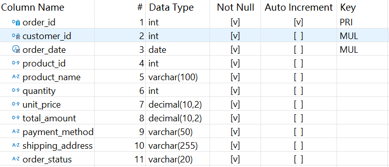
A MySQL database contains the orders_30m table, which stores historical order data spanning multiple years. The table structure is as follows:

Sample data:

1 3001 2023-01-05 701 Smartphone Z 1 699.99 699.99 Credit Card 888 Eighth St, Charlotte, NC Delivered

2 3002 2023-02-10 702 Smart Scale 1 49.99 49.99 PayPal 999 Ninth Ave, Indianapolis, IN Delivered

3 3003 2023-03-15 703 Laptop Air 1 1099.99 1099.99 Credit Card 101 Tenth Rd, Seattle, WA Delivered

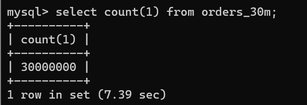
Data volume: 30 million rows.

Two sample queries:

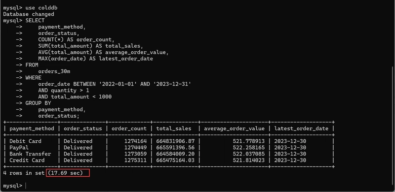
Analyze 2022-2023 sales by payment method and order status:

SELECT 
    payment_method,
    order_status,
    COUNT(*) AS order_count,
    SUM(total_amount) AS total_sales,
    AVG(total_amount) AS average_order_value,
    MAX(order_date) AS latest_order_date
FROM 
    orders
WHERE 
    order_date BETWEEN '2022-01-01' AND '2023-12-31'
    AND quantity > 1  
    AND total_amount < 1000  
GROUP BY 
    payment_method, 
    order_status;

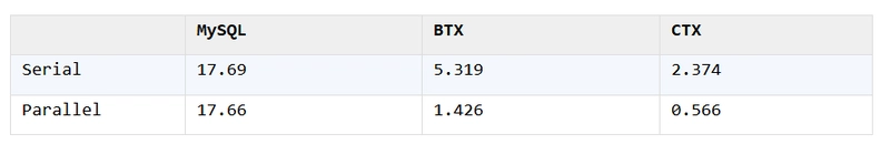
Query time: 17.69 seconds.

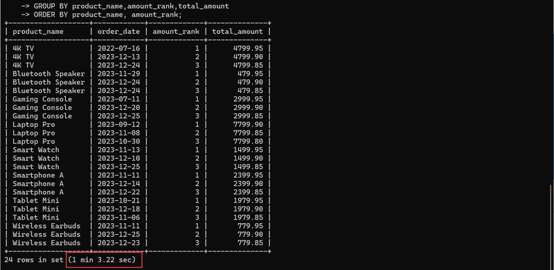
Find the top 3 orders by total amount for each product category:

WITH ranked_orders AS (
    SELECT 
        product_name,
        order_id,
        customer_id,
        order_date,
        total_amount,
        DENSE_RANK() OVER (
            PARTITION BY product_name
            ORDER BY total_amount DESC
        ) AS amount_rank
    FROM 
        orders
)
SELECT * FROM ranked_orders
WHERE amount_rank <= 3
ORDER BY product_name, amount_rank;

Query time: 63.22 seconds.

Now we use esProc to dump the data into files to speed up queries.

Installing esProc
First, download esProc Standard Edition ,It's free.

After installation, configure a connection to the MySQL database.

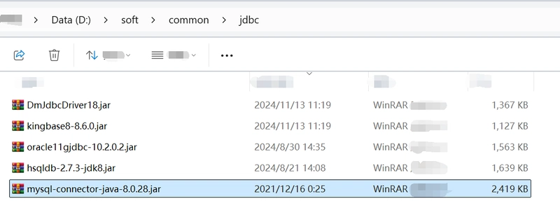
Begin by placing the MySQL JDBC driver package in the directory [esProc installation directory]\common\jdbc (similar setup for other databases).

Then, start the esProc IDE. From the menu bar, select Tool > Connect to Data Source and configure a standard MySQL JDBC connection.

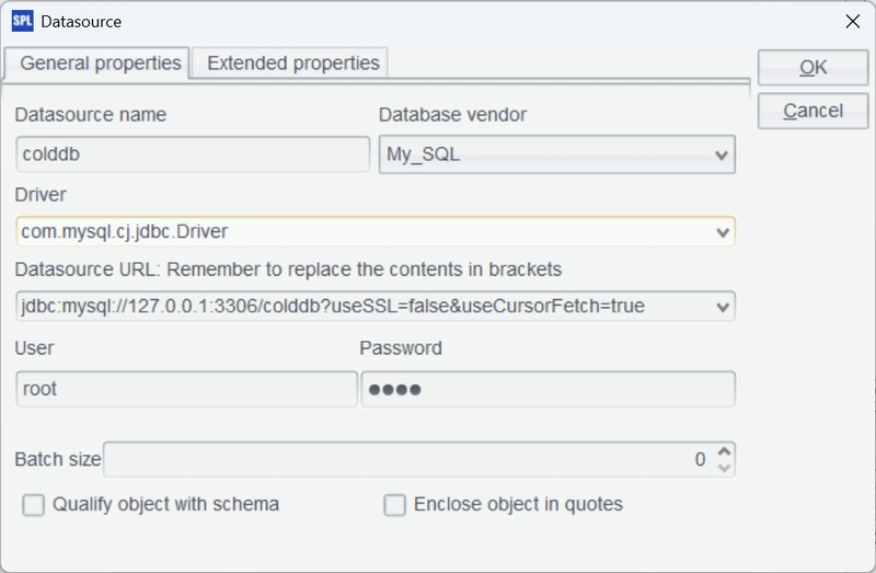
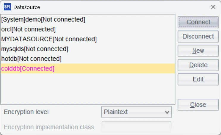
After confirming the settings, test the connection by clicking “Connect”. If the colddb data source just configured turns pink, the connection is successful.

Dump data to BTX
Next, export the orders table to a binary row-based file with the .btx extension.

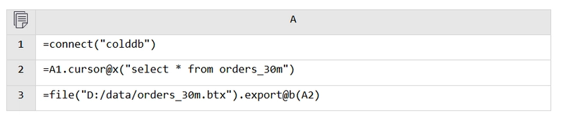
Generating the BTX file is simple – simply export the data. Because of the large data volume, A2 uses a cursor, which can handle data of any scale.

Press Ctrl+F9 to execute:

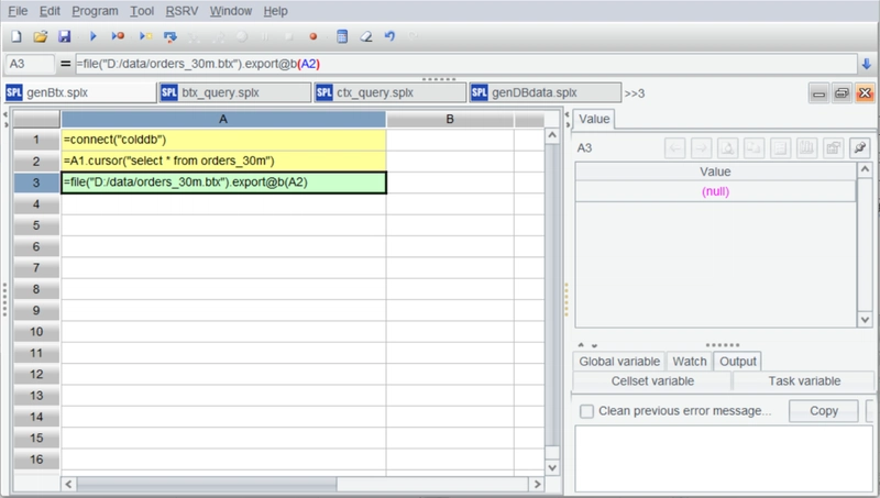
The BTX file is now generated:

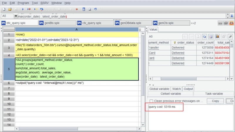
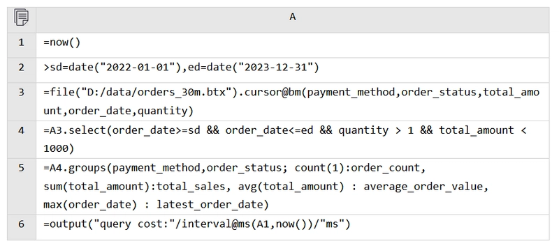
Now, let’s perform the first calculation described earlier—analyze 2022-2023 sales by payment method and order status—using the BTX file.

A3 creates a file cursor, reading only the necessary columns. A4 uses select for conditional filtering, and A5 performs grouping and aggregation. The code is straightforward and requires no further explanation.

Running the code yields the correct results with a query time of 5.319 seconds, 3.3 times faster than MySQL.

Dump data to CTX
In addition to BTX, esProc also offers a lightweight columnar binary file format CTX. Let’s try converting the orders table to CTX.

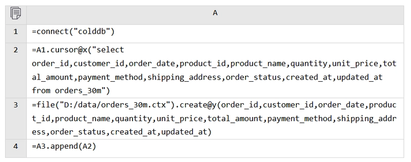
When creating a CTX file, it first needs to define the data structure (A3), which should be identical to that of the orders table. A4 then writes the data into the CTX file.
It can be seen that the columnar CTX file achieves a significantly higher compression ratio than the row-based BTX file.

Now, let’s repeat the first calculation.

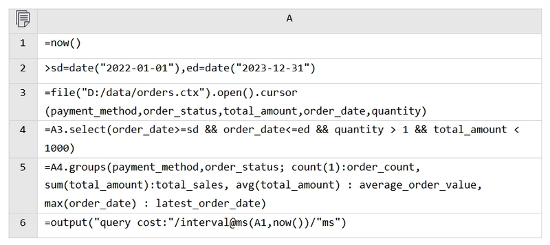
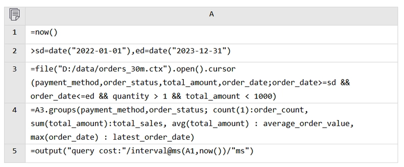
To use CTX, it first needs to open the file and then create a cursor. The remaining code is identical to that used with BTX.

Execution time: 3.061 seconds, which is faster than BTX.

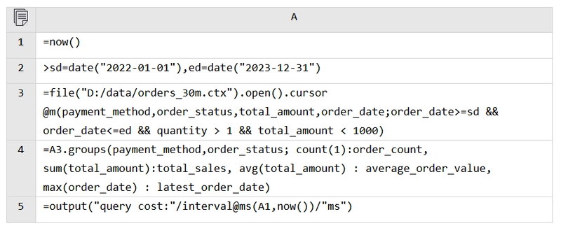
CTX also offers ‘cursor filtering’, an optimization technique. By adding the filter conditions to the cursor, esProc first reads only the values of the fields used in the conditions. If a condition is not met, esProc skips to the next record; otherwise, it reads the remaining required fields and creates the record.

In A3, the filter conditions are placed on the cursor, and the rest of the code remains essentially the same.

Execution time: 2.374 seconds.

Here, the filter conditions use 3 fields, while the total number of fields read is only 5. Therefore, the performance improvement is only 32%. If the difference in the number of fields were greater, the performance difference would be more significant.

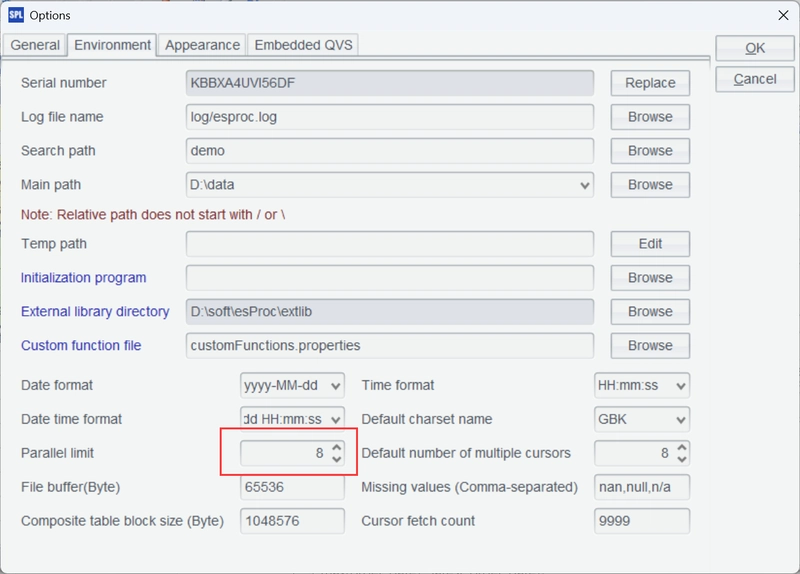
Parallel computation
esProc also makes it easy to write parallel code for both BTX and CTX files; simple set the number of parallel threads to match the CPU core count (8 cores are configured here).

Here is the script for parallel computation with BTX:

By simply adding the @m option after the cursor enables esProc to automatically perform parallel computation based on the configured number of threads, making it very convenient.

Execution time: 1.426 seconds.

The process is similar for CTX:

Adding the @m option reduces the execution time to 0.566 seconds.

Of course, many databases also support parallel computation. However, MySQL’s performance in this regard seems to be less effective. Even after setting the parallel parameters, there was no significant performance improvement.

The following table summarizes the execution times for the tests described above (in seconds):

For the above-mentioned second calculation involving in-group TopN, detailed test results are not provided here. The file-based approach is still much faster (single-threaded: 63.22/2.075=30.5 times faster). The esProc code implementation, shown below, demonstrates its concise and elegant syntax.

Find the top 3 orders by total amount for each product category:

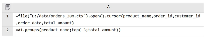
esProc simplifies TopN implementation by treating it as an aggregation operation.

In conclusion, both file formats of esProc are faster than databases, especially the CTX file. Common operations can be several to a dozen times faster, while more complex TopN operations can be tens of times faster. Therefore, dumping data to files offers significant advantages. However, file storage has its specific applicable scenarios. Because it requires exporting data, it’s more suitable for calculations on static historical data, which are common. To process new data, esProc’s mixed computation capabilities are required, but these are beyond the scope of this discussion. Please visit the official website for further details.