High-Performance Location Searching: How Map Apps Handle Billions of Places

When you open a map application and start typing "coffee shop near me," you get instant results showing nearby locations. This seemingly simple search is actually an impressive technical feat. Behind the scenes, finding locations among billions of possible places across the globe requires sophisticated engineering solutions. Let's explore how major mapping platforms like Google Maps, Apple Maps, and Waze achieve this remarkable performance. The Challenge of Global Location Search Scale: Map applications need to index hundreds of millions of businesses, landmarks, streets, and points of interest worldwide Realtime updates: New businesses open, others close, and roads change constantly Complex queries: Users want to find places by name, category, proximity, ratings, and other attributes Low latency: Results must appear almost instantly to provide a good user experience Accuracy: False negatives mean users can't find what they're looking for Let's dive into the data structures and techniques that make this possible. Geospatial Hash Tables:Making Location Lookups Lightning Fast At the heart of fast location searching is the geospatial hash table. Unlike traditional hash maps that store simple key-value pairs, geospatial hash tables are optimized for coordinates and location data. When you search for "coffee shop," the system doesn't scan the entire global database. Instead, it uses a technique called "geohashing" to convert coordinates into compact string representations that preserve locality. Nearby locations share similar geohash prefixes, making regional searches incredibly efficient. For example, the coordinates of downtown Seattle might be encoded as "c23nb," while nearby Pike Place Market might be "c23nf." This encoding allows systems to quickly retrieve all locations within a geographic area by searching for entries with matching prefixes. Geohashing transforms the two-dimensional problem of spatial proximity into a one-dimensional string comparison, achieving lookups in nearly constant time regardless of the total number of locations in the system. Quadtrees and R-trees: Organizing Spatial Data Hierarchically While geohashing works well for many queries, mapping applications also rely on specialized tree structures for more complex spatial operations. Quadtrees divide geographic space into hierarchical quadrants. Starting with the entire globe, each region is recursively split into four equal parts until reaching an appropriate level of detail. This creates a tree where each node represents a geographic area, and its children represent subdivisions of that area. When you're zooming into a map, the application traverses down this tree structure, efficiently loading only the data for the visible region. R-trees take a different approach, focusing on minimum bounding rectangles (MBRs) that contain geographic objects. This structure excels at range queries like "find all restaurants within this neighborhood" because it can quickly eliminate large portions of the dataset that fall outside the query area. The key advantage of these tree structures is their O(log n) search performance. Even with billions of locations worldwide, finding all points in a specific area might only require examining a handful of nodes in the tree. Spatial Indexes in Databases: Making Geography Queryable Traditional database indexes like B-trees work well for one-dimensional data but struggle with geographical coordinates. To solve this, modern spatial databases implement specialized spatial indexes. PostGIS (PostgreSQL's spatial extension) and MongoDB's geospatial indexes use variations of R-trees to accelerate location queries. These indexes organize data points by their geographical proximity, ensuring that "nearest neighbor" searches complete in logarithmic rather than linear time. Google's S2 library takes this further by mapping Earth's surface onto a three-dimensional cube, then using space-filling curves to convert positions into one-dimensional index values. This approach allows extremely fast "nearest" queries while preserving spatial relationships. The power of spatial indexes becomes evident when searching across massive datasets. Finding the 10 nearest coffee shops among millions of businesses takes just milliseconds, regardless of how many total places exist in the database. Bloom Filters: Rapid Elimination of Non-Matches When users perform searches like "vegan bakery open now," mapping applications need to quickly filter through millions of businesses. Bloom filters provide a probabilistic way to eliminate non-matches almost instantly. A Bloom filter is a space-efficient data structure that tells you if an item is definitely not in a set or might be in a set. It never produces false negatives but can occasionally produce false positives. Map applications maintain multiple bloom filters for different attributes: one might check if businesses are open at certain hours, another might filter by cat

Apr 26, 2025 - 16:58

High-Performance Location Searching: How Map Apps Handle Billions of Places

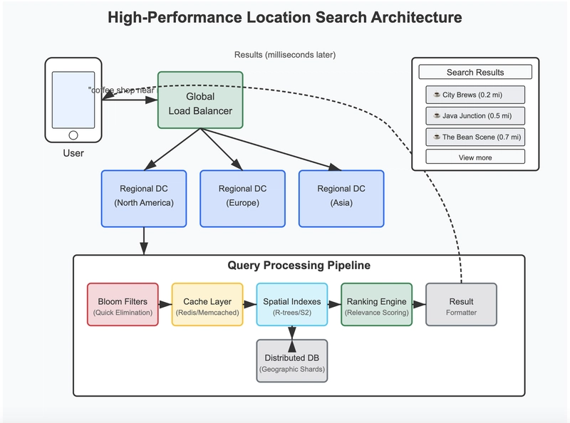
When you open a map application and start typing "coffee shop near me," you get instant results showing nearby locations. This seemingly simple search is actually an impressive technical feat. Behind the scenes, finding locations among billions of possible places across the globe requires sophisticated engineering solutions. Let's explore how major mapping platforms like Google Maps, Apple Maps, and Waze achieve this remarkable performance.

The Challenge of Global Location Search

Scale: Map applications need to index hundreds of millions of businesses, landmarks, streets, and points of interest worldwide
Realtime updates: New businesses open, others close, and roads change constantly
Complex queries: Users want to find places by name, category, proximity, ratings, and other attributes
Low latency: Results must appear almost instantly to provide a good user experience
Accuracy: False negatives mean users can't find what they're looking for Let's dive into the data structures and techniques that make this possible. Geospatial Hash Tables:Making Location Lookups Lightning Fast At the heart of fast location searching is the geospatial hash table. Unlike traditional hash maps that store simple key-value pairs, geospatial hash tables are optimized for coordinates and location data.

When you search for "coffee shop," the system doesn't scan the entire global database. Instead, it uses a technique called "geohashing" to convert coordinates into compact string representations that preserve locality. Nearby locations share similar geohash prefixes, making regional searches incredibly efficient.

For example, the coordinates of downtown Seattle might be encoded as "c23nb," while nearby Pike Place Market might be "c23nf." This encoding allows systems to quickly retrieve all locations within a geographic area by searching for entries with matching prefixes.

Geohashing transforms the two-dimensional problem of spatial proximity into a one-dimensional string comparison, achieving lookups in nearly constant time regardless of the total number of locations in the system.

Quadtrees and R-trees: Organizing Spatial Data Hierarchically
While geohashing works well for many queries, mapping applications also rely on specialized tree structures for more complex spatial operations.

*Quadtrees divide geographic space into hierarchical quadrants. *
Starting with the entire globe, each region is recursively split into four equal parts until reaching an appropriate level of detail. This creates a tree where each node represents a geographic area, and its children represent subdivisions of that area.

When you're zooming into a map, the application traverses down this tree structure, efficiently loading only the data for the visible region.

R-trees take a different approach, focusing on minimum bounding rectangles (MBRs) that contain geographic objects. This structure excels at range queries like "find all restaurants within this neighborhood" because it can quickly eliminate large portions of the dataset that fall outside the query area.

The key advantage of these tree structures is their O(log n) search performance. Even with billions of locations worldwide, finding all points in a specific area might only require examining a handful of nodes in the tree.

Spatial Indexes in Databases: Making Geography Queryable
Traditional database indexes like B-trees work well for one-dimensional data but struggle with geographical coordinates. To solve this, modern spatial databases implement specialized spatial indexes.

PostGIS (PostgreSQL's spatial extension) and MongoDB's geospatial indexes use variations of R-trees to accelerate location queries. These indexes organize data points by their geographical proximity, ensuring that "nearest neighbor" searches complete in logarithmic rather than linear time.

Google's S2 library takes this further by mapping Earth's surface onto a three-dimensional cube, then using space-filling curves to convert positions into one-dimensional index values. This approach allows extremely fast "nearest" queries while preserving spatial relationships.

The power of spatial indexes becomes evident when searching across massive datasets. Finding the 10 nearest coffee shops among millions of businesses takes just milliseconds, regardless of how many total places exist in the database.

Bloom Filters: Rapid Elimination of Non-Matches
When users perform searches like "vegan bakery open now," mapping applications need to quickly filter through millions of businesses. Bloom filters provide a probabilistic way to eliminate non-matches almost instantly.

A Bloom filter is a space-efficient data structure that tells you if an item is definitely not in a set or might be in a set. It never produces false negatives but can occasionally produce false positives.

Map applications maintain multiple bloom filters for different attributes: one might check if businesses are open at certain hours, another might filter by category, and so on. When a query arrives, the system runs it through these filters first.

For example, when searching for "vegan restaurants," the bloom filter can immediately eliminate 99% of locations that definitely don't match this category. Only potential matches proceed to more expensive verification steps.

With just a few megabytes of memory, a bloom filter can represent essential attributes of millions of places, drastically reducing the computational load on search systems.

In-Memory Caching: Keeping Hot Data Close
Map applications receive millions of similar queries. People frequently search for popular landmarks, chain restaurants, and major transportation hubs. To handle this efficiently, they implement sophisticated caching strategies.

Redis and Memcached serve as high-performance caching layers, storing precomputed results for common queries. These in-memory systems can respond in microseconds, far faster than even the most optimized database operations.

The caching strategy typically follows these principles:

Locality-based caching: Each geographic region maintains its own cache of popular searches
Time-aware expiration: Results for queries like "open now" expire more quickly than stable data
Hierarchical caching: Results are cached at different geographic scales (neighborhood, city, region)

When you search for "coffee shop" in a major city, chances are someone nearby has made a similar query recently. The system can return cached results instantly while refreshing them in the background.

Distributed Architecture: Scaling to Global Proportions
No single machine could handle the load of a global mapping service. Instead, the architecture distributes data and processing across thousands of servers.

Google Maps, for example, shards its data geographically. Queries for locations in Tokyo are routed to servers specializing in Japanese data, while searches in Chicago go to North American clusters.

This geographic sharding strategy offers several advantages:

Lower latency: Users connect to servers physically closer to them
Regional relevance: Data and search algorithms can be tuned for regional patterns
Fault isolation: Issues affecting one region don't impact the entire system Each regional cluster maintains its own set of bloom filters, spatial indexes, and caches optimized for local queries. Load balancers at both global and local levels ensure smooth traffic distribution.

Bringing It All Together: The Search Pipeline

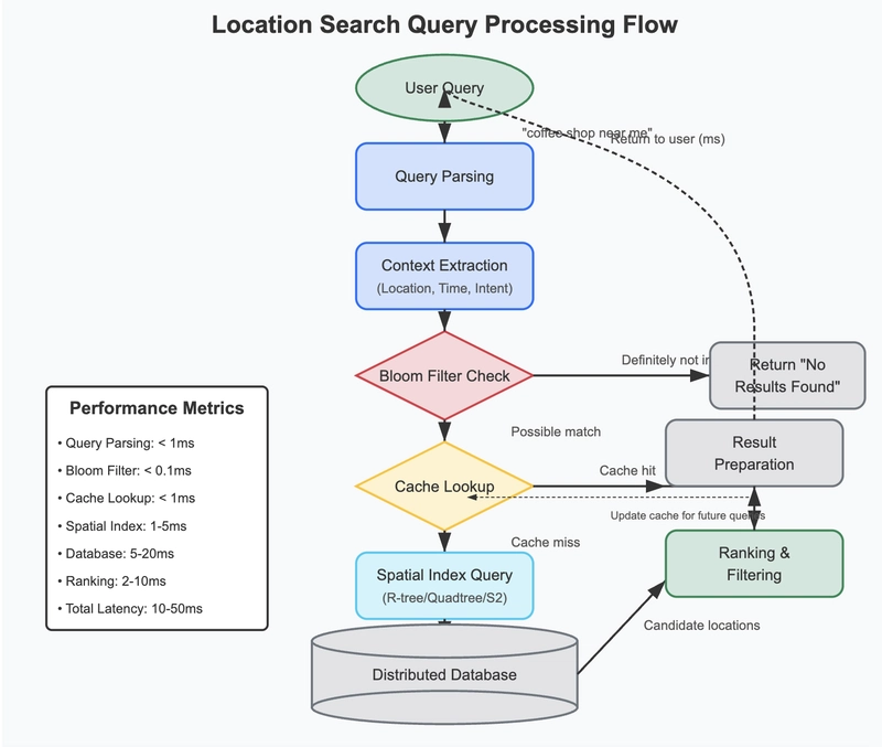
When you type "pizza delivery open now" into a mapping app, here's what typically happens:

Request routing: A global load balancer directs your query to the appropriate regional data center
Query parsing: The system extracts key components (business type, attributes, location context)
Bloom filter check: Bloom filters quickly eliminate locations that definitely don't match
Cache lookup: The system checks if identical or similar queries have recent results
Spatial index query: For new searches, spatial indexes find candidates in the relevant area
Ranking and filtering: Remaining candidates are scored and filtered based on relevance
Result preparation: The top matches are formatted with necessary details for display

This entire process completes in milliseconds, giving you the impression of instant results despite the enormous dataset being searched.

Conclusion
The next time you quickly find a restaurant or navigate to a new address, remember the sophisticated technology working behind the scenes. From bloom filters and geospatial hash tables to distributed caching and specialized tree structures, location search represents a masterful application of computer science principles.

By strategically combining these techniques, map applications can search through billions of places worldwide and still return relevant results in milliseconds. It's a testament to how clever data structures and system design can solve incredibly complex problems while providing a seamless user experience.