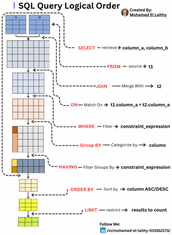
SQL Query Logical Order

SQL Query Logical Order: A Step-by-Step Breakdown Understanding the logical execution order of an SQL query is essential for writing optimized and efficient database queries. Unlike the typical SQL syntax order, the execution follows a systematic approach. Here's a breakdown: FROM – Identifying the Data Source The query execution starts by selecting the main table (t1) from which data will be retrieved. This step lays the foundation for subsequent operations. JOIN – Merging Tables If multiple tables are involved, the JOIN operation merges another table (t2) based on specified conditions, preparing a unified dataset for filtering and processing. ON – Defining Match Conditions The ON clause establishes the conditions for the JOIN, ensuring the correct records are linked, typically using a primary-foreign key relationship (e.g., t1.column_a = t2.column_a). WHERE – Filtering Rows The WHERE clause applies constraints to filter rows before any aggregation or grouping occurs, enhancing query performance by reducing unnecessary computations. GROUP BY – Categorizing Data Data is then grouped based on a specific column, enabling aggregate functions like COUNT(), SUM(), and AVG() to operate on each group efficiently. HAVING – Filtering Groups Unlike WHERE, which filters individual rows, HAVING filters grouped results based on conditions like HAVING COUNT(*) > 10. ORDER BY – Sorting the Results The query results are then sorted in ascending (ASC) or descending (DESC) order based on one or more columns, ensuring structured output. LIMIT – Restricting the Output Finally, the LIMIT clause restricts the number of rows returned, optimizing performance and preventing unnecessary data retrieval.

Mar 16, 2025 - 12:23

SQL Query Logical Order: A Step-by-Step Breakdown
Understanding the logical execution order of an SQL query is essential for writing optimized and efficient database queries. Unlike the typical SQL syntax order, the execution follows a systematic approach. Here's a breakdown:

FROM – Identifying the Data Source
The query execution starts by selecting the main table (t1) from which data will be retrieved. This step lays the foundation for subsequent operations.
JOIN – Merging Tables
If multiple tables are involved, the JOIN operation merges another table (t2) based on specified conditions, preparing a unified dataset for filtering and processing.
ON – Defining Match Conditions
The ON clause establishes the conditions for the JOIN, ensuring the correct records are linked, typically using a primary-foreign key relationship (e.g., t1.column_a = t2.column_a).
WHERE – Filtering Rows
The WHERE clause applies constraints to filter rows before any aggregation or grouping occurs, enhancing query performance by reducing unnecessary computations.
GROUP BY – Categorizing Data
Data is then grouped based on a specific column, enabling aggregate functions like COUNT(), SUM(), and AVG() to operate on each group efficiently.
HAVING – Filtering Groups
Unlike WHERE, which filters individual rows, HAVING filters grouped results based on conditions like HAVING COUNT(*) > 10.
ORDER BY – Sorting the Results
The query results are then sorted in ascending (ASC) or descending (DESC) order based on one or more columns, ensuring structured output.
LIMIT – Restricting the Output
Finally, the LIMIT clause restricts the number of rows returned, optimizing performance and preventing unnecessary data retrieval.